8 Wage Analytics - Predicting High vs. Low Earners Using Logistic Regression
8.1 Chapter Introduction
This assignment investigates wage outcomes using the Wage dataset from the ISLR package. We categorize wages into High and Low groups based on the median and aim to identify factors associated with higher earnings.
The analysis demonstrates:
- Descriptive comparisons of wage groups by age and education.
- Group differences using t-tests and ANOVA.
- Association tests using Chi-Square and effect size (Cramer’s V).
- Predictive modeling using logistic regression, including evaluation with confusion matrices and ROC/AUC.
This chapter illustrates how demographic, job-related, and health variables contribute to wage outcomes and demonstrates predictive modeling for classification.
data("Wage", package = "ISLR")
w <- Wage


# Create wage category based on the median
med_wage <- median(w$wage, na.rm = TRUE)
w <- w %>%
dplyr::mutate(
WageCategory = dplyr::case_when(
wage > med_wage ~ "High",
wage < med_wage ~ "Low",
TRUE ~ NA_character_
),
WageCategory = factor(WageCategory, levels = c("Low", "High"))
)


table(w$WageCategory, useNA = "ifany")
#>
#>  Low High <NA>
#> 1447 1483   70
fix_factor_prefix <- function(f) {
lv <- levels(f)
lv <- gsub("^[0-9]+-", "", lv)
levels(f) <- lv
f
}


factor_vars <- names(w)[sapply(w, is.factor)]


for (v in factor_vars) {
w[[v]] <- fix_factor_prefix(w[[v]])
}
age_by_wage <- w %>%
  dplyr::filter(!is.na(WageCategory)) %>%
  dplyr::select(age, WageCategory)


age_summary <- age_by_wage %>%
  dplyr::group_by(WageCategory) %>%
  dplyr::summarise(
    mean_age = mean(age, na.rm = TRUE),
    n = dplyr::n()
  )


age_summary
#> # A tibble: 2 × 3
#>   WageCategory mean_age     n
#>   <fct>           <dbl> <int>
#> 1 Low              40.0  1447
#> 2 High             44.7  1483


t_res <- t.test(age ~ WageCategory, data = age_by_wage)
broom::tidy(t_res)
#> # A tibble: 1 × 10
#>   estimate estimate1 estimate2 statistic  p.value parameter
#>      <dbl>     <dbl>     <dbl>     <dbl>    <dbl>     <dbl>
#> 1    -4.67      40.0      44.7     -11.1 3.14e-28     2725.
#> # ℹ 4 more variables: conf.low <dbl>, conf.high <dbl>,
#> # method <chr>, alternative <chr>8.3 Test statistics
- t = -11.14
- df = 2724.7
- p < 2.2 x 10^-16
8.3.1 Interpretation
There is a statistically significant age difference between High and Low wage earners. On average, High earners are about 4.7 years older than Low earners. Because the p-value is extremely small, we conclude that age is meaningfully associated with earning a high wage in this dataset.
aov_mod <- aov(wage ~ education, data = w)
summary(aov_mod)
#>               Df  Sum Sq Mean Sq F value Pr(>F)
#> education      4 1226364  306591   229.8 <2e-16 ***
#> Residuals   2995 3995721    1334
#> ---
#> Signif. codes:
#> 0 '***' 0.001 '**' 0.01 '*' 0.05 '.' 0.1 ' ' 1


TukeyHSD(aov_mod)
#>   Tukey multiple comparisons of means
#>     95% family-wise confidence level
#>
#> Fit: aov(formula = wage ~ education, data = w)
#>
#> $education
#>                                        diff       lwr
#> 2. HS Grad-1. < HS Grad            11.67894  4.799846
#> 3. Some College-1. < HS Grad       23.65115 16.413966
#> 4. College Grad-1. < HS Grad       40.32349 33.140488
#> 5. Advanced Degree-1. < HS Grad    66.81336 59.040518
#> 3. Some College-2. HS Grad         11.97221  6.919816
#> 4. College Grad-2. HS Grad         28.64456 23.670077
#> 5. Advanced Degree-2. HS Grad      55.13443 49.340723
#> 4. College Grad-3. Some College    16.67234 11.213367
#> 5. Advanced Degree-3. Some College 43.16221 36.947555
#> 5. Advanced Degree-4. College Grad 26.48987 20.338392
#>                                         upr    p adj
#> 2. HS Grad-1. < HS Grad            18.55803 3.68e-05
#> 3. Some College-1. < HS Grad       30.88834 0.00e+00
#> 4. College Grad-1. < HS Grad       47.50650 0.00e+00
#> 5. Advanced Degree-1. < HS Grad    74.58621 0.00e+00
#> 3. Some College-2. HS Grad         17.02461 0.00e+00
#> 4. College Grad-2. HS Grad         33.61904 0.00e+00
#> 5. Advanced Degree-2. HS Grad      60.92813 0.00e+00
#> 4. College Grad-3. Some College    22.13132 0.00e+00
#> 5. Advanced Degree-3. Some College 49.37687 0.00e+00
#> 5. Advanced Degree-4. College Grad 32.64134 0.00e+00
8.4 From the ANOVA table
- F(4, 2995) = 229.8
- p < 2 x 10^-16
8.4.1 Interpretation
There is a significant effect of education level on wage. Individuals with higher levels of education earn significantly higher wages on average. Tukey post-hoc comparisons show that every education level differs significantly from the one below it, with wages increasing steadiy from “<HS Grad” up to “Advanced Degree.” Education appears to be one of the strongest predictors of wage in the dataset.
ct <- table(w$WageCategory, w$jobclass)
ct
#>
#>        1. Industrial 2. Information
#>   Low            878            569
#>   High           629            854


chisq_res <- chisq.test(ct)
chisq_res
#>
#>  Pearson's Chi-squared test with Yates' continuity
#>  correction
#>
#> data:  ct
#> X-squared = 97.065, df = 1, p-value < 2.2e-16


CramerV(ct)
#> [1] 0.1826937
8.5 Test statistics
- X^2 = 97.07
- df = 1
- p < 2.2 x 10^-16
- Cramer’s V = 0.183 (small-medium association)
8.5.1 Interpreation
Wage catergory is significantly associated with type of job class. - Low earners are more common in Industrial jobs. - High earners are more common in Information jobs. Although the association is not extremely strong (V≈0.18), it is meaningful and indicates job class plays a role in wage outcomes.
set.seed(2025)
split <- caTools::sample.split(w$WageCategory, SplitRatio = 0.70)
train_data <- w[split, ]
test_data <- w[!split, ]


prop.table(table(train_data$WageCategory))
#>
#>       Low      High
#> 0.4939054 0.5060946
prop.table(table(test_data$WageCategory))
#>
#>       Low      High
#> 0.4937429 0.5062571
train_data <- train_data %>%
dplyr::mutate(
education = droplevels(education),
jobclass = droplevels(jobclass),
maritl = droplevels(maritl),
race = droplevels(race),
health = droplevels(health),
health_ins = droplevels(health_ins)
)


logit_mod <- glm(
WageCategory ~ age + education + jobclass + maritl + race + health + health_ins + year,
data = train_data,
family = binomial
)


summary(logit_mod)
#>
#> Call:
#> glm(formula = WageCategory ~ age + education + jobclass + maritl +
#>     race + health + health_ins + year, family = binomial, data = train_data)
#>
#> Coefficients:
#>                               Estimate Std. Error z value
#> (Intercept)                 -1.843e+02  5.361e+01  -3.439
#> age                          2.310e-02  5.461e-03   4.230
#> education2. HS Grad          5.113e-01  2.186e-01   2.339
#> education3. Some College     1.381e+00  2.270e-01   6.080
#> education4. College Grad     2.279e+00  2.307e-01   9.879
#> education5. Advanced Degree  2.837e+00  2.631e-01  10.781
#> jobclass2. Information       4.450e-02  1.117e-01   0.398
#> maritl2. Married             1.244e+00  1.549e-01   8.033
#> maritl3. Widowed             8.607e-01  7.734e-01   1.113
#> maritl4. Divorced            5.827e-01  2.482e-01   2.348
#> maritl5. Separated           4.309e-01  4.516e-01   0.954
#> race2. Black                -5.851e-01  1.914e-01  -3.057
#> race3. Asian                -7.874e-02  2.300e-01  -0.342
#> race4. Other                -9.274e-02  4.685e-01  -0.198
#> health2. >=Very Good         2.443e-01  1.206e-01   2.025
#> health_ins2. No             -1.237e+00  1.228e-01 -10.074
#> year                         9.038e-02  2.672e-02   3.382
#>                             Pr(>|z|)
#> (Intercept)                 0.000585 ***
#> age                         2.34e-05 ***
#> education2. HS Grad         0.019349 *
#> education3. Some College    1.20e-09 ***
#> education4. College Grad     < 2e-16 ***
#> education5. Advanced Degree  < 2e-16 ***
#> jobclass2. Information      0.690321
#> maritl2. Married            9.50e-16 ***
#> maritl3. Widowed            0.265812
#> maritl4. Divorced           0.018856 *
#> maritl5. Separated          0.339988
#> race2. Black                0.002234 **
#> race3. Asian                0.732111
#> race4. Other                0.843081
#> health2. >=Very Good        0.042871 *
#> health_ins2. No              < 2e-16 ***
#> year                        0.000720 ***
#> ---
#> Signif. codes:
#> 0 '***' 0.001 '**' 0.01 '*' 0.05 '.' 0.1 ' ' 1
#>
#> (Dispersion parameter for binomial family taken to be 1)
#>
#>     Null deviance: 2843.0  on 2050  degrees of freedom
#> Residual deviance: 2117.3  on 2034  degrees of freedom
#> AIC: 2151.3
#>
#> Number of Fisher Scoring iterations: 4


odds_table <- broom::tidy(logit_mod, exponentiate = TRUE, conf.int = TRUE)
knitr::kable(odds_table, digits = 3)| term | estimate | std.error | statistic | p.value | conf.low | conf.high |
|---|---|---|---|---|---|---|
| (Intercept) | 0.000 | 53.609 | -3.439 | 0.001 | 0.000 | 0.000 |
| age | 1.023 | 0.005 | 4.230 | 0.000 | 1.013 | 1.034 |
| education2. HS Grad | 1.667 | 0.219 | 2.339 | 0.019 | 1.095 | 2.586 |
| education3. Some College | 3.977 | 0.227 | 6.080 | 0.000 | 2.570 | 6.270 |
| education4. College Grad | 9.768 | 0.231 | 9.879 | 0.000 | 6.272 | 15.518 |
| education5. Advanced Degree | 17.059 | 0.263 | 10.781 | 0.000 | 10.292 | 28.908 |
| jobclass2. Information | 1.046 | 0.112 | 0.398 | 0.690 | 0.839 | 1.301 |
| maritl2. Married | 3.470 | 0.155 | 8.033 | 0.000 | 2.568 | 4.715 |
| maritl3. Widowed | 2.365 | 0.773 | 1.113 | 0.266 | 0.518 | 11.296 |
| maritl4. Divorced | 1.791 | 0.248 | 2.348 | 0.019 | 1.100 | 2.912 |
| maritl5. Separated | 1.539 | 0.452 | 0.954 | 0.340 | 0.617 | 3.662 |
| race2. Black | 0.557 | 0.191 | -3.057 | 0.002 | 0.381 | 0.808 |
| race3. Asian | 0.924 | 0.230 | -0.342 | 0.732 | 0.590 | 1.456 |
| race4. Other | 0.911 | 0.469 | -0.198 | 0.843 | 0.348 | 2.218 |
| health2. >=Very Good | 1.277 | 0.121 | 2.025 | 0.043 | 1.008 | 1.618 |
| health_ins2. No | 0.290 | 0.123 | -10.074 | 0.000 | 0.228 | 0.369 |
| year | 1.095 | 0.027 | 3.382 | 0.001 | 1.039 | 1.154 |
8.6 Significant predictors
- Age
- Education: all levels 2-5
- Married, divorced
- Race: Black
- Health: ≥Very Good
- Health insurance: No
- Year
8.8 Direction and size (using Odds Ratios)
-
Education is the strongest predictor. For example:
- Advanced Degree OR = 17.06 -College Grade OR = 9.77
- Age: OR = 1.023 -> each additional year increases odds of High wage by ~2.3%.
- Married: OR = 3.47 -> much higher offs of being a High earner.
- Race (Black): OR = 0.56 -> lower odds of hgih wage compared to White.
- No health insurance: OR = 0.29 -> surprisingly strong decrease in odds.
- Year: OR = 1.095 -> later survey years have higher odds of high wages.
8.9 Findings
Job class was not significant, even though the Chi-square test showed an association. This often happens when other stronger variables absorb the predictive power. Also, individuals without health insurance had much lower odds of high wage, which may reflect socioeconomic or employer-benefit differences.
test_data$pred_prob <- predict(logit_mod, newdata = test_data, type = "response")


test_data$pred_class <- factor(
ifelse(test_data$pred_prob >= 0.5, "High", "Low"),
levels = c("Low", "High")
)


confusionMatrix(test_data$pred_class, test_data$WageCategory, positive = "High")
#> Confusion Matrix and Statistics
#>
#>           Reference
#> Prediction Low High
#>       Low  325  126
#>       High 109  319
#>
#>                Accuracy : 0.7327
#>                  95% CI : (0.7021, 0.7617)
#>     No Information Rate : 0.5063
#>     P-Value [Acc > NIR] : <2e-16
#>
#>                   Kappa : 0.4655
#>
#>  Mcnemar's Test P-Value : 0.2966
#>
#>             Sensitivity : 0.7169
#>             Specificity : 0.7488
#>          Pos Pred Value : 0.7453
#>          Neg Pred Value : 0.7206
#>              Prevalence : 0.5063
#>          Detection Rate : 0.3629
#>    Detection Prevalence : 0.4869
#>       Balanced Accuracy : 0.7329
#>
#>        'Positive' Class : High
#>
8.10 Confusion matrix results
- Accuracy: 0.733
- Sensitivity (High earners detected): 0.717
- Specificity (Low earners detected): 0.749
- Balanced Accuracy: 0.733
- No Information Rate (NIR): 0.506
- Accuracy is much higher than the NIR, and p<2e-16 confirms the model significantly beats chance.
8.10.1 Interpretation
The model performs well on unseen data. It predicts both wage categories reasonably well, with slightly stronger performance for Low earners (higher specificity). Overall accuracy is strong relative to the baseline.
roc_obj <- roc(
response = test_data$WageCategory,
predictor = test_data$pred_prob,
levels = c("Low", "High"),
direction = "<"
)


auc_val <- auc(roc_obj)
auc_val
#> Area under the curve: 0.8196


plot(roc_obj, main = paste0("ROC Curve (AUC = ", round(auc_val, 3), ")"))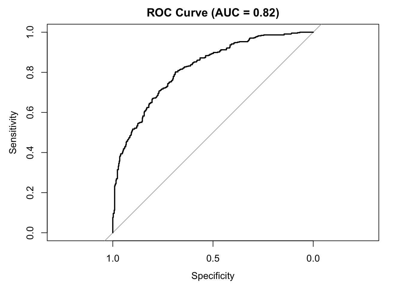
Figure 8.1: ROC curve for logistic regression model predicting High wage earners. AUC = 0.82 indicates excellent discrimination between High and Low earners.
- AUC = 0.820
- An AUC aboce 0.80 indicates excellent classification performance.
8.10.2 Interpreation
The ROC curve shows the model is effective at distinguishing High vs. Low earners. Sensitivity (correctly identifying High earners) is strong, and specificity is also good. The AUC well exceeds the chance level of 0.50, and accuracy is far above the NIR, confirming that the model performs reliably better than random guessing.
8.11 Final Interpretation
The results across descriptive statistics, group comparisons, and predictive modeling all suggest that wage outcomes are systematically related to age, education, marital status, and job-related characteristics. Age shows a notable difference between wage groups, with High earners being significantly older on average. Education emerges as one of the most significant correlates of wage, confirmed by both ANOVA and logistic regression. Wages consistently increase as educational attainment rises, and each step up from “<HS” to “Advanced Degree” adds a considerable wage increase.
Job class also demonstrates an association with wage category in the Chi-square analysis, with Information jobs containing a higher proportion of High earners. However, when included alongside other predictors in the logistic regression, job class is no longer a significant predictor. This suggests that job class and wage category are linked, but much of the predictive value is explained by other variables, such as education. Marital status also plays a notable role; married individuals have substantially higher odds of being High earners, while divorce offers a smaller and significant increase.
The logistic regression model provided strong predictive performance. Accuracy on the test set (73.3%) was well above the No Information Rate (50.6%), and the AUC of 0.82 shows excellent ability to discriminate between High and Low earners. The model predicted Low earners slightly more accurately, but performance was balanced overall. These results indicate that the model generalizes well to unseen data and captures meaningful patterns in the wage structure.
If this analysis were repeated, it might be valuable to add variables related to type of industry, years of experience, workload, or employer characteristics, which might further clarify wage drivers. Removing non-significant predictors like job class or some of the race categories might slightly simplify the model without harming predictive power. Overall, the results emphasize the strong importance of education, marital status, age, and health insurance status in predicting wage category within the Wage dataset.