2 R Script to R Markdown Report
2.1 Introduction
This report explores the NYPD Shooting Incidents Data using R. The workflow demonstrates how to acquire, clean, and visualize open-source data in a reproducible way.
2.3 Loading the Data
# API call to NYC Open Data
url <- "https://data.cityofnewyork.us/resource/833y-fsy8.json"
shooting_data <- jsonlite::fromJSON(url)

# Peek at data
head(shooting_data)
#>   incident_key              occur_date occur_time     boro
#> 1    298699604 2024-12-31T00:00:00.000   19:16:00 BROOKLYN
#> 2    298699604 2024-12-31T00:00:00.000   19:16:00 BROOKLYN
#> 3    298672096 2024-12-30T00:00:00.000   16:45:00    BRONX
#> 4    298672096 2024-12-30T00:00:00.000   16:45:00    BRONX
#> 5    298672095 2024-12-30T00:00:00.000   20:32:00    BRONX
#> 6    298672096 2024-12-30T00:00:00.000   16:45:00    BRONX
#>   loc_of_occur_desc precinct jurisdiction_code
#> 1           OUTSIDE       69                 0
#> 2           OUTSIDE       69                 0
#> 3           OUTSIDE       47                 0
#> 4           OUTSIDE       47                 0
#> 5            INSIDE       41                 0
#> 6           OUTSIDE       47                 0
#>   loc_classfctn_desc           location_desc
#> 1             STREET                  (null)
#> 2             STREET                  (null)
#> 3             STREET                  (null)
#> 4             STREET                  (null)
#> 5           DWELLING MULTI DWELL - APT BUILD
#> 6             STREET                  (null)
#>   statistical_murder_flag perp_age_group perp_sex perp_race
#> 1                   FALSE          25-44        M     BLACK
#> 2                   FALSE          25-44        M     BLACK
#> 3                   FALSE         (null)   (null)    (null)
#> 4                   FALSE         (null)   (null)    (null)
#> 5                    TRUE          18-24        M     BLACK
#> 6                   FALSE         (null)   (null)    (null)
#>   vic_age_group vic_sex       vic_race x_coord_cd
#> 1         18-24       M          BLACK  1,015,120
#> 2         25-44       M          BLACK  1,015,120
#> 3           <18       F WHITE HISPANIC  1,021,316
#> 4         25-44       F WHITE HISPANIC  1,021,316
#> 5         25-44       M          BLACK  1,012,201
#> 6         18-24       M          BLACK  1,021,316
#>   y_coord_cd  latitude  longitude geocoded_column.type
#> 1    173,870 40.643866 -73.888761                Point
#> 2    173,870 40.643866 -73.888761                Point
#> 3    259,277 40.878261 -73.865964                Point
#> 4    259,277 40.878261 -73.865964                Point
#> 5    240,878 40.827795 -73.899003                Point
#> 6    259,277 40.878261 -73.865964                Point
#>   geocoded_column.coordinates :@computed_region_yeji_bk3q
#> 1         -73.88876, 40.64387                           2
#> 2         -73.88876, 40.64387                           2
#> 3         -73.86596, 40.87826                           5
#> 4         -73.86596, 40.87826                           5
#> 5           -73.8990, 40.8278                           5
#> 6         -73.86596, 40.87826                           5
#>   :@computed_region_92fq_4b7q :@computed_region_sbqj_enih
#> 1                           8                          42
#> 2                           8                          42
#> 3                           2                          30
#> 4                           2                          30
#> 5                          43                          25
#> 6                           2                          30
#>   :@computed_region_efsh_h5xi :@computed_region_f5dn_yrer
#> 1                       13827                           5
#> 2                       13827                           5
#> 3                       11605                          29
#> 4                       11605                          29
#> 5                       10937                          34
#> 6                       11605                          29
The dataset currently contains 1000 rows of shooting incident records.
2.4 Data Cleaning
shooting_clean <- shooting_data %>%
  # Step 1: Remove rows missing occur_date
  filter(!is.na(occur_date)) %>%
  # Step 2: Create time_of_day variable
  mutate(
    occur_date = ymd(occur_date),
    occur_time = hm(occur_time),
    hour = hour(occur_time),
    time_of_day = case_when(
      hour >= 5 & hour < 12 ~ "Morning",
      hour >= 12 & hour < 17 ~ "Afternoon",
      hour >= 17 & hour < 21 ~ "Evening",
      TRUE ~ "Night"
    ),
    borough = str_to_title(boro)
  )
#> Warning: There were 2 warnings in `mutate()`.
#> The first warning was:
#> ℹ In argument: `occur_date = ymd(occur_date)`.
#> Caused by warning:
#> ! All formats failed to parse. No formats found.
#> ℹ Run `dplyr::last_dplyr_warnings()` to see the 1 remaining
#>   warning.
I cleaned the dataset by dropping rows with missing dates, creating a time_of_day variable based on the hour of the incident, and standardizing borough names.
2.5 Insights
# Distribution of incidents by borough
borough_counts <- shooting_clean %>%
  count(borough, sort = TRUE)

borough_counts
#>         borough   n
#> 1         Bronx 366
#> 2      Brooklyn 296
#> 3     Manhattan 190
#> 4        Queens 137
#> 5 Staten Island  11
The table above shows the distribution of incidents across boroughs. The borough with the most shootings is Bronx.
# Create a clean table with kable
kable(borough_counts, caption = "Distribution of Shooting Incidents by Borough")| borough | n |
|---|---|
| Bronx | 366 |
| Brooklyn | 296 |
| Manhattan | 190 |
| Queens | 137 |
| Staten Island | 11 |
2.6 Visualizations
ggplot(shooting_clean, aes(x = time_of_day)) +
geom_bar(fill = "steelblue") +
labs(title = "Shooting Incidents by Time of Day",
x = "Time of Day",
y = "Count of Incidents") +
theme_minimal()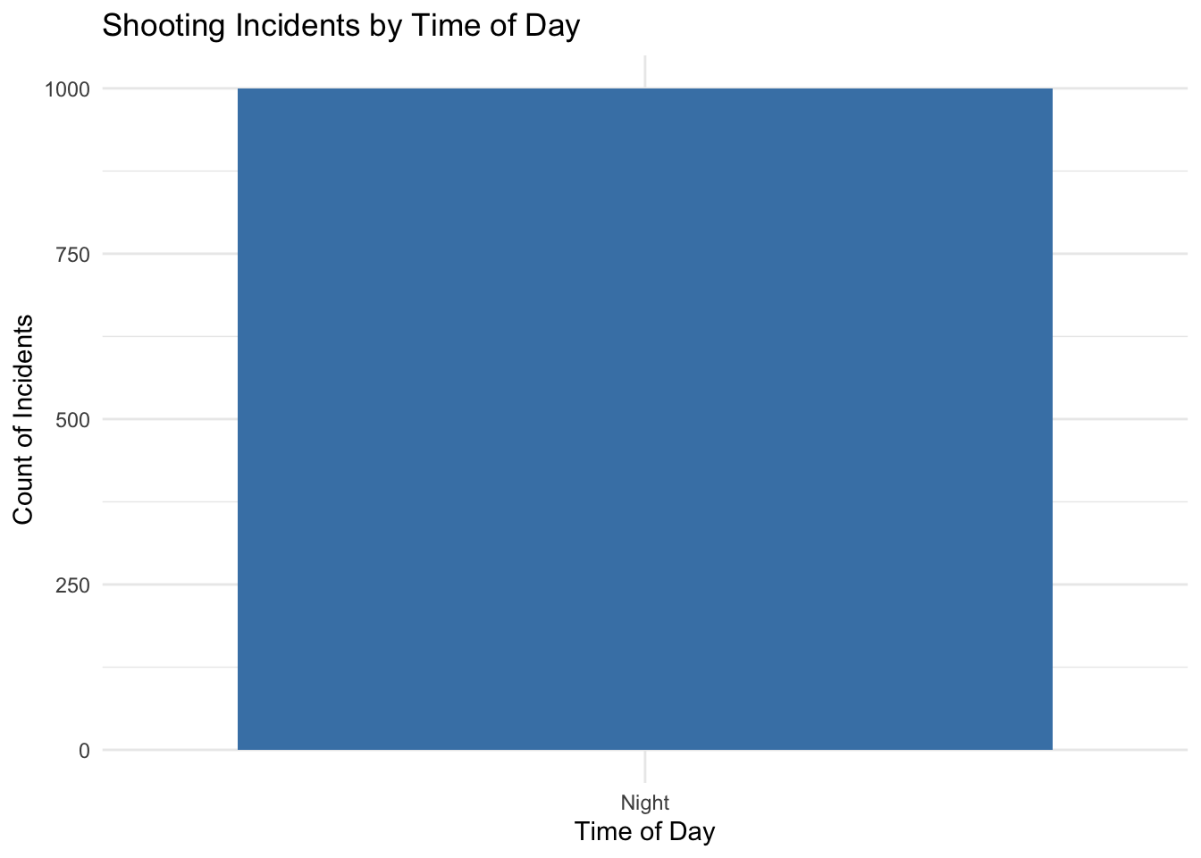 The bar plot above shows how shootings are distributed across different times of the day.
ggplot(shooting_clean, aes(x = borough)) +
geom_bar(fill = "darkred") +
labs(title = "Shooting Incidents by Borough",
x = "Borough",
y = "Count of Incidents") +
theme_minimal()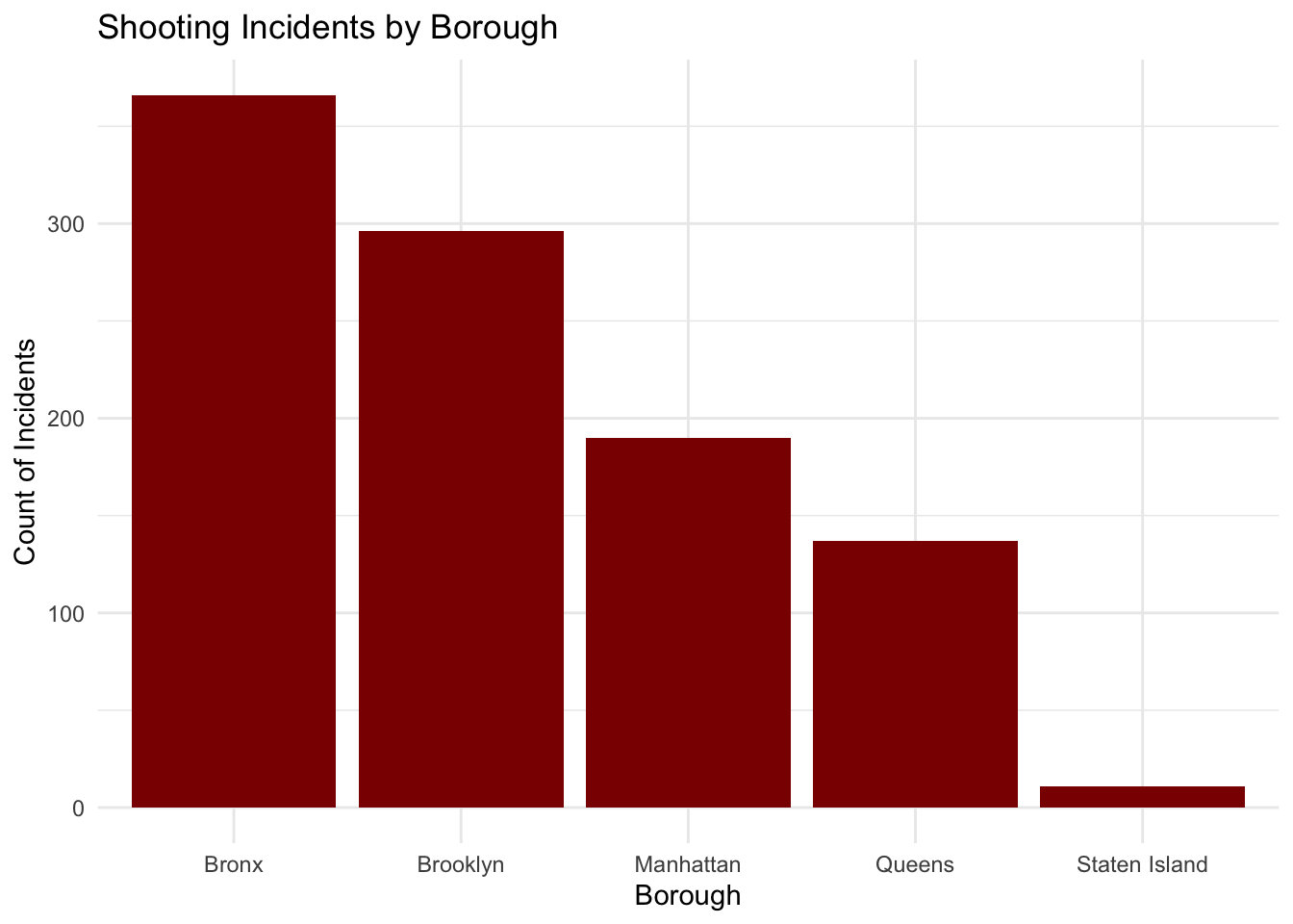 The second plot shows which boroughs experience the highest number of incidents.
2.7 Reflection
Learning R Markdown this week has shown me how to keep my code and explanations together in one place, which helps make my work easier to follow. I can see how this would help me with my thesis on climate change and peer anxiety/influence because I’ll be able to keep track of my analysis steps and show exactly how I got my results. It also makes me think more carefully about how to explain what the numbers and graphs mean and not just how to calculate them. Using R Markdown has helped me also learn the best ways to share my results and findings with others.