5 NBA Analytics - Exploring Team Performance Through Reproducible Analysis
5.1 Chapter Introduction
This chapter analyzes NBA team performance during the 2024-2025 season using reproducible data analysis techniques in R. The goal of the assignment is to explore relationships between offensive production, defensive activity, player age, and conference affiliation. Skills demonstrated include data wrangling across multiple Excel sheets, visualization with ggplot2, correlation analysis, and statistical interpretation. All analyses are conducted at the team level, which is important to consider when interpreting results.
5.3 Data Import and Cleaning
# File names
team_xlsx <- "NBA Team Total Data 2024-2025.xlsx"
conf_xlsx <- "Team Conferences.xlsx"

# Check all sheet names in the team data workbook
excel_sheets(team_xlsx)
#>  [1] "Nets"         "Knicks"       "Raptors"
#>  [4] "Philly"       "Celtics"      "Timberwolves"
#>  [7] "Thunder"      "Jazz"         "Trailblazers"
#> [10] "Nuggets"      "Bulls"        "Bucks"
#> [13] "Cavaliers"    "Pistons"      "Pacers"
#> [16] "Warriors"     "Suns"         "Lakers"
#> [19] "Clippers"     "Kings"        "Hornets"
#> [22] "Magic"        "Wizards"      "Hawks"
#> [25] "Heat"         "Grizzles"     "Spurs"
#> [28] "Pelicans"     "Rockets"      "Mavericks"
library(readxl)

# Look at the first team sheet to check the column names
test_sheet <- read_excel(team_xlsx, sheet = 1)
names(test_sheet)
#>  [1] "Rk"      "Player"  "Age"     "G"       "GS"
#>  [6] "MP"      "FG"      "FGA"     "FG%"     "3P"
#> [11] "3PA"     "3P%"     "2P"      "2PA"     "2P%"
#> [16] "eFG%"    "FT"      "FTA"     "FT%"     "ORB"
#> [21] "DRB"     "TRB"     "AST"     "STL"     "BLK"
#> [26] "TOV"     "PF"      "PTS"     "Trp-Dbl" "Awards"
# Function to load each team’s data
load_team_data <- function(sheet_name) {
  df <- read_excel(team_xlsx, sheet = sheet_name)

  df <- df %>%
    mutate(
      Team = sheet_name,
      Won_award = ifelse(Awards > 0, 1, 0),
      PRA = PTS + TRB + AST,
      STOCKS = STL + BLK
    )

  return(df)
}

# Apply the function to all sheets and combine
all_teams <- lapply(excel_sheets(team_xlsx), load_team_data) %>%
  bind_rows()

# Preview combined dataset
head(all_teams)
#> # A tibble: 6 × 35
#>      Rk Player       Age     G    GS    MP    FG   FGA `FG%`
#>   <dbl> <chr>      <dbl> <dbl> <dbl> <dbl> <dbl> <dbl> <dbl>
#> 1     1 Jalen Wil…    24    79    22  2031   246   620 0.397
#> 2     2 Keon John…    22    79    56  1925   303   779 0.389
#> 3     3 Nic Claxt…    25    70    62  1882   320   568 0.563
#> 4     4 Cameron J…    28    57    57  1800   355   747 0.475
#> 5     5 Ziaire Wi…    23    63    45  1541   214   520 0.412
#> 6     6 Tyrese Ma…    25    60    11  1315   189   465 0.406
#> # ℹ 26 more variables: `3P` <dbl>, `3PA` <dbl>,
#> #   `3P%` <dbl>, `2P` <dbl>, `2PA` <dbl>, `2P%` <dbl>,
#> #   `eFG%` <dbl>, FT <dbl>, FTA <dbl>, `FT%` <dbl>,
#> #   ORB <dbl>, DRB <dbl>, TRB <dbl>, AST <dbl>, STL <dbl>,
#> #   BLK <dbl>, TOV <dbl>, PF <dbl>, PTS <dbl>,
#> #   `Trp-Dbl` <dbl>, Awards <chr>, Team <chr>,
#> #   Won_award <dbl>, PRA <dbl>, STOCKS <dbl>, Pos <chr>
# Load the conference lookup data
conference_lookup <- read_excel(conf_xlsx)

# Merge with main dataset and create binary variable
all_teams <- all_teams %>%
  left_join(conference_lookup, by = "Team") %>%
  mutate(Conference_binary = ifelse(Conference == "East", 1, 0))

# Preview to confirm
head(all_teams)
#> # A tibble: 6 × 37
#>      Rk Player       Age     G    GS    MP    FG   FGA `FG%`
#>   <dbl> <chr>      <dbl> <dbl> <dbl> <dbl> <dbl> <dbl> <dbl>
#> 1     1 Jalen Wil…    24    79    22  2031   246   620 0.397
#> 2     2 Keon John…    22    79    56  1925   303   779 0.389
#> 3     3 Nic Claxt…    25    70    62  1882   320   568 0.563
#> 4     4 Cameron J…    28    57    57  1800   355   747 0.475
#> 5     5 Ziaire Wi…    23    63    45  1541   214   520 0.412
#> 6     6 Tyrese Ma…    25    60    11  1315   189   465 0.406
#> # ℹ 28 more variables: `3P` <dbl>, `3PA` <dbl>,
#> #   `3P%` <dbl>, `2P` <dbl>, `2PA` <dbl>, `2P%` <dbl>,
#> #   `eFG%` <dbl>, FT <dbl>, FTA <dbl>, `FT%` <dbl>,
#> #   ORB <dbl>, DRB <dbl>, TRB <dbl>, AST <dbl>, STL <dbl>,
#> #   BLK <dbl>, TOV <dbl>, PF <dbl>, PTS <dbl>,
#> #   `Trp-Dbl` <dbl>, Awards <chr>, Team <chr>,
#> #   Won_award <dbl>, PRA <dbl>, STOCKS <dbl>, Pos <chr>, …
5.4 Visualizations
fig.cap="Scatterplot showing the relationship between offensive performance (PRA) and defensive activity (STOCKS), colored by conference. Each point represents a team, allowing comparison of overall team balance across conferences. The boxplot below displays the distribution of PRA values within each conference, highlighting variability and central tendencies in offensive production."
# Scatterplot: PRA vs STOCKS by Conference
ggplot(all_teams, aes(x = PRA, y = STOCKS, color = Conference)) +
  geom_point(size = 3) +
  labs(
    title = "Offensive vs. Defensive Performance by Conference",
    x = "Points + Rebounds + Assists (PRA)",
    y = "Steals + Blocks (STOCKS)",
    color = "Conference"
  ) +
  theme_minimal()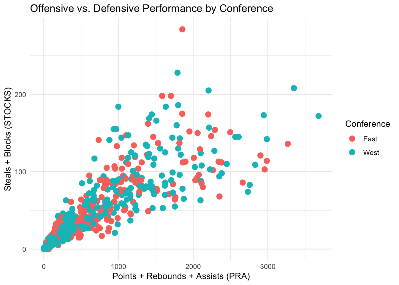
# Second visualization: average PRA by Conference
ggplot(all_teams, aes(x = Conference, y = PRA, fill = Conference)) +
geom_boxplot() +
labs(
title = "Distribution of PRA by Conference",
x = "Conference",
y = "PRA (Offensive Metric)"
) +
theme_minimal()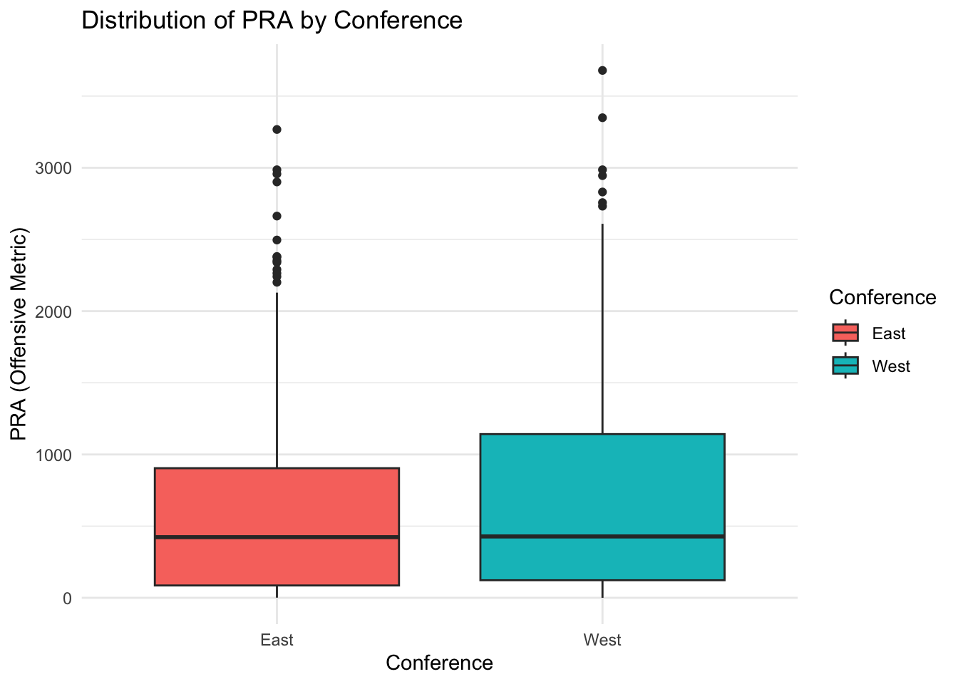 These figures visualize how teams balance offensive and defensive output and whether conference affiliation appears related to overall performance patterns.
5.5 Correlation Analysis
# Point-biserial correlations (Conference vs PRA and STOCKS)
cor.test(all_teams$Conference_binary, all_teams$PRA)
#>
#>  Pearson's product-moment correlation
#>
#> data:  all_teams$Conference_binary and all_teams$PRA
#> t = -1.8195, df = 650, p-value = 0.0693
#> alternative hypothesis: true correlation is not equal to 0
#> 95 percent confidence interval:
#>  -0.147164250  0.005629906
#> sample estimates:
#>         cor
#> -0.07118475
cor.test(all_teams$Conference_binary, all_teams$STOCKS)
#>
#>  Pearson's product-moment correlation
#>
#> data:  all_teams$Conference_binary and all_teams$STOCKS
#> t = -2.094, df = 650, p-value = 0.03665
#> alternative hypothesis: true correlation is not equal to 0
#> 95 percent confidence interval:
#>  -0.157650363 -0.005105577
#> sample estimates:
#>         cor
#> -0.08185737

# Create correlation matrix for Age, PRA, and STOCKS
corr_data <- all_teams %>%
  dplyr::select(Age, PRA, STOCKS) %>%
  na.omit()

# Compute and visualize correlation matrix
corr_matrix <- cor(corr_data)
ggcorrplot(corr_matrix, lab = TRUE, title = "Correlation Matrix: Age, PRA, and STOCKS")
#> Warning: `aes_string()` was deprecated in ggplot2 3.0.0.
#> ℹ Please use tidy evaluation idioms with `aes()`.
#> ℹ See also `vignette("ggplot2-in-packages")` for more
#>   information.
#> ℹ The deprecated feature was likely used in the ggcorrplot
#>   package.
#>   Please report the issue at
#>   <https://github.com/kassambara/ggcorrplot/issues>.
#> This warning is displayed once every 8 hours.
#> Call `lifecycle::last_lifecycle_warnings()` to see where
#> this warning was generated.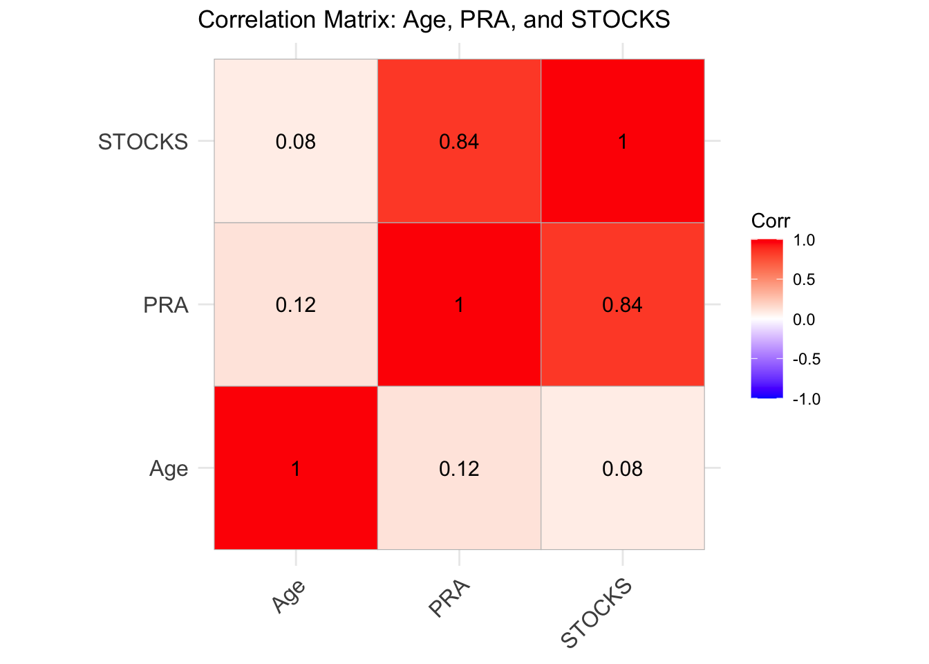
Figure 5.1: Correlation matrix illustrating the relationships among Age, PRA, and STOCKS
This analysis examiness whether team age profiles are associated with offensive and defensive performance metrics.
5.6 Executive Memo
#>
#> **To:** NBA Commissioner Adam Silver
#> **From:** Emma Valentina Tupone
#> **Subject:** Summary of 2024-2025 Team Performance Analysis
#>
#> Our analysis of team performance metrics shows a moderate positive relationship between offensive output (Points + Rebounds + Assists, PRA) and defensive activity (Steals + Blocks, STOCKS).
#> Teams that performed well offensively tended to also perform well defensively.
#>
#> Overall, differences between Eastern and Western Conference teams were minor. There was also no strong evidence that one conference consistently outperformed the other across these measures.
#>
#> When focusing on player Age, the relationship between PRA and STOCKS remained positive. This suggests that team performance links are not primarily driven by player experience.
#>
#> **Limitation:** The data represents team-level totals rather than individual player-level performance, limiting insight into specific player contributions.
#> **Next Step:** Future analyses could include player efficiency ratings or advanced metrics such as plus-minus to better understand what drives elite performances across teams.