3 Law Firm Analysis
3.1 Chapter Introduction
In this assignment, we analyze New York City violation data to understand patterns in payment amounts for parking and camera tickets. The goal is to uncover differences across issuing agencies, driver states, and counties that could inform a law firm’s strategy for contesting tickets or targeting marketing efforts.
We use descriptive statistics, visualizations, and inferential analyses (ANOVA) to answer the following questions:
- Do certain issuing agencies issue higher payments?
- Do drivers from the tri-state area (NY, NJ, CT) pay more?
- Do certain counties tend to have higher payment amounts?
The dataset comes from the NYC Open Data Portal.
This chapter demonstrates data cleaning, data manipulation, visualization, and statistical analysis skills in R using real-world city data.
3.3 Load and Prepare the Data
# Download from NYC API
if (file.exists("camera_data.RData")) {
  load("camera_data.RData")
  message("Loaded local dataset: camera_data.RData")
} else {
  message("Downloading dataset from NYC Open Data...")
  endpoint <- "https://data.cityofnewyork.us/resource/nc67-uf89.json"
  resp <- GET(endpoint, query = list("$limit" = 99999, "$order" = "issue_date DESC"))
  camera <- fromJSON(content(resp, as = "text"), flatten = TRUE)
  save(camera, file = "camera_data.RData")
  message("Saved dataset locally as camera_data.RData")
}
#> Loaded local dataset: camera_data.RData

# Confirm structure
glimpse(camera)
#> Rows: 99,999
#> Columns: 20
#> $ plate                     <chr> "HPK2083", "FFZ7198", "B…
#> $ state                     <chr> "NY", "NY", "99", "99", …
#> $ license_type              <chr> "PAS", "PAS", "999", "99…
#> $ summons_number            <chr> "1420103131", "140579752…
#> $ violation_time            <chr> "00:00A", "06:49A", NA, …
#> $ violation                 <chr> "INSP. STICKER-EXPIRED/M…
#> $ fine_amount               <chr> "65", "95", "45", "0", "…
#> $ penalty_amount            <chr> "0", "0", "0", "0", "0",…
#> $ interest_amount           <chr> "0", "0", "0", "0", "0",…
#> $ reduction_amount          <chr> "65", "95", "45", "0", "…
#> $ payment_amount            <chr> "0", "0", "0", "0", "0",…
#> $ amount_due                <chr> "0", "0", "0", "0", "0",…
#> $ precinct                  <chr> "025", "000", "104", "00…
#> $ issuing_agency            <chr> "POLICE DEPARTMENT", "PO…
#> $ county                    <chr> NA, "Q", NA, "Q", NA, "Q…
#> $ violation_status          <chr> NA, "HEARING HELD-NOT GU…
#> $ issue_date                <chr> NA, NA, NA, NA, NA, NA, …
#> $ judgment_entry_date       <chr> NA, NA, NA, NA, NA, NA, …
#> $ summons_image.url         <chr> "http://nycserv.nyc.gov/…
#> $ summons_image.description <chr> "View Summons", "View Su…

# Convert numeric variables
camera <- camera %>%
  mutate(across(
    c("fine_amount","interest_amount","reduction_amount","payment_amount",
      "amount_due","penalty_amount"),
    ~as.numeric(.)
  ))

# Filter valid dates
camera <- camera %>%
  filter(str_detect(issue_date, "^\\d{4}-\\d{2}-\\d{2}T"))
camera$issue_date <- as.Date(camera$issue_date)
3.4 Issuing Agency and Payment Amount
3.4.1 Visualization
ggplot(camera, aes(x = issuing_agency, y = payment_amount)) +
  geom_boxplot(fill = "steelblue", color = "gray30") +
  coord_flip() +
  theme_minimal() +
  labs(title = "Payment Amount by Issuing Agency",
       x = "Issuing Agency", y = "Payment Amount ($)")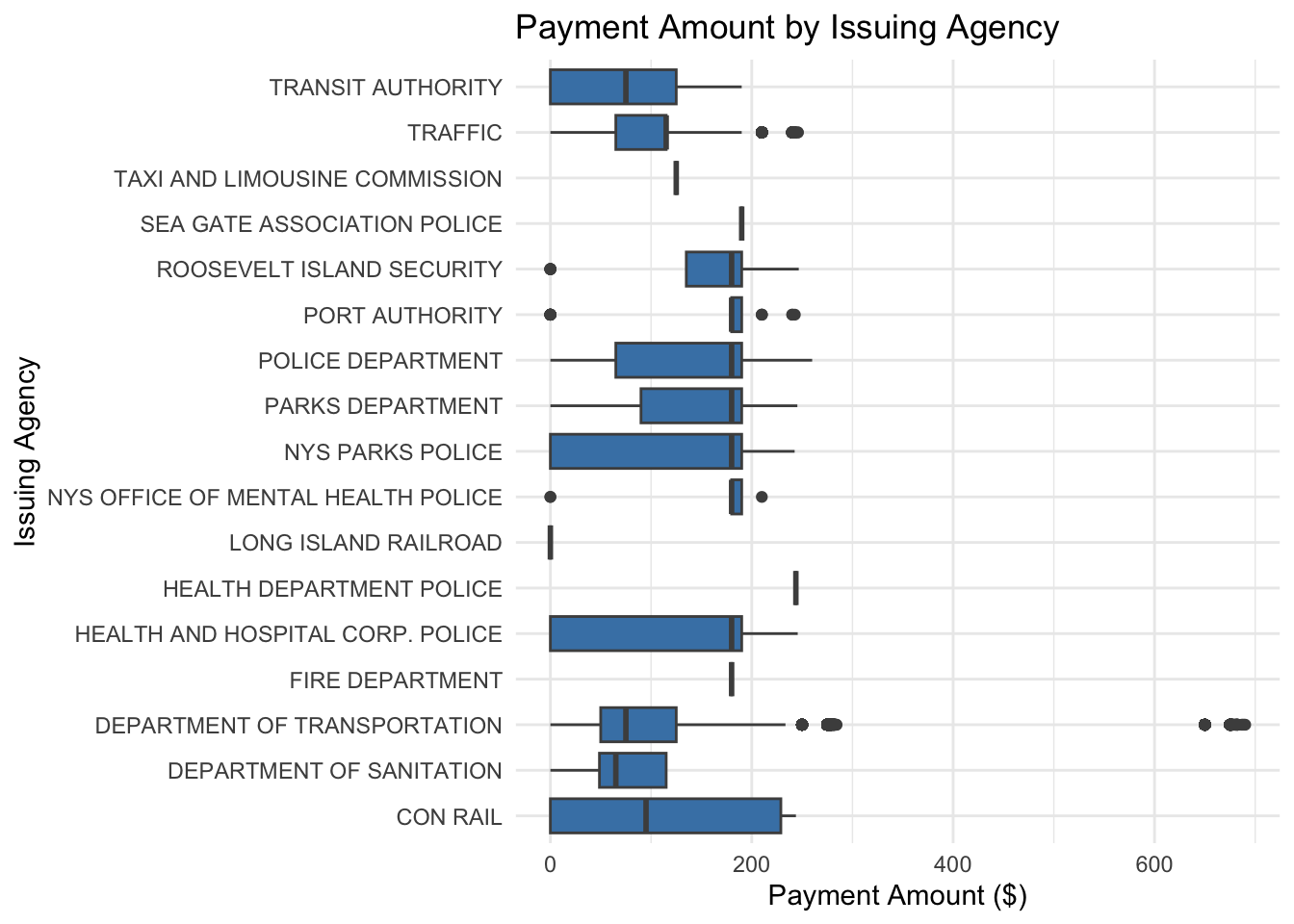
Figure 3.1: Boxplot showing distribution of payment amounts for each issuing agency. Each box represents the median, interquartile range, and potential outliers, allowing comparison of payment patterns across agencies.
3.4.2 Descriptive Statistics
favstats(payment_amount ~ issuing_agency, data = camera) %>%
  arrange(desc(mean))
#>                        issuing_agency    min     Q1 median
#> 1            HEALTH DEPARTMENT POLICE 243.81 243.81 243.81
#> 2         SEA GATE ASSOCIATION POLICE 190.00 190.00 190.00
#> 3                     FIRE DEPARTMENT 180.00 180.00 180.00
#> 4  NYS OFFICE OF MENTAL HEALTH POLICE   0.00 180.00 180.00
#> 5                      PORT AUTHORITY   0.00 180.00 180.00
#> 6           ROOSEVELT ISLAND SECURITY   0.00 135.00 180.00
#> 7                    NYS PARKS POLICE   0.00   0.00 180.00
#> 8                   POLICE DEPARTMENT   0.00  65.00 180.00
#> 9                    PARKS DEPARTMENT   0.00  90.00 180.00
#> 10      TAXI AND LIMOUSINE COMMISSION 125.00 125.00 125.00
#> 11   HEALTH AND HOSPITAL CORP. POLICE   0.00   0.00 180.00
#> 12                           CON RAIL   0.00   0.00  95.00
#> 13       DEPARTMENT OF TRANSPORTATION   0.00  50.00  75.00
#> 14                            TRAFFIC   0.00  65.00 115.00
#> 15                  TRANSIT AUTHORITY   0.00   0.00  75.00
#> 16           DEPARTMENT OF SANITATION   0.00  48.75  65.00
#> 17               LONG ISLAND RAILROAD   0.00   0.00   0.00
#>          Q3    max      mean        sd     n missing
#> 1  243.8100 243.81 243.81000        NA     1       0
#> 2  190.0000 190.00 190.00000   0.00000     2       0
#> 3  180.0000 180.00 180.00000        NA     1       0
#> 4  190.0000 210.00 161.33333  65.99423    15       0
#> 5  190.0000 242.76 150.49319  80.53742    47       0
#> 6  190.0000 246.68 149.16083  90.57967    24       0
#> 7  190.0000 242.58 142.50970  90.27092    33       0
#> 8  190.0000 260.00 136.71574  82.82498   190       0
#> 9  190.0000 245.28 128.47736  78.92728   144       0
#> 10 125.0000 125.00 125.00000        NA     1       0
#> 11 190.0000 245.64 124.71373  98.60130    51       0
#> 12 228.8875 243.87 112.62000 124.87146     6       0
#> 13 125.0000 690.04  99.52822  82.88394 87273       0
#> 14 115.0000 245.79  94.59362  44.47453 12091       0
#> 15 125.0000 190.00  78.00000  82.05181     5       0
#> 16 115.0000 115.00  66.25000  45.48351    12       0
#> 17   0.0000   0.00   0.00000        NA     1       0
3.4.3 Inferential Statistics
anova_agency <- aov(payment_amount ~ issuing_agency, data = camera)
summary(anova_agency)
#>                   Df    Sum Sq Mean Sq F value Pr(>F)
#> issuing_agency    16   1063435   66465   10.59 <2e-16 ***
#> Residuals      99880 627060364    6278
#> ---
#> Signif. codes:
#> 0 '***' 0.001 '**' 0.01 '*' 0.05 '.' 0.1 ' ' 1
supernova(anova_agency)
#>  Analysis of Variance Table (Type III SS)
#>  Model: payment_amount ~ issuing_agency
#>
#>                                     SS    df        MS
#>  ----- --------------- | ------------- ----- ---------
#>  Model (error reduced) |   1063434.678    16 66464.667
#>  Error (from model)    | 627060364.280 99880  6278.137
#>  ----- --------------- | ------------- ----- ---------
#>  Total (empty model)   | 628123798.957 99896  6287.777
#>       F   PRE     p
#>  ------ ----- -----
#>  10.587 .0017 .0000
#>
#>  ------ ----- -----
#>
3.4.4 Interpretation
If the F-value is large and p < .05, there are statistically significant differences in mean payment amounts between issuing agencies.
Though, the PRE (Proportion Reduction in Error) shows how much variance is explained. A small PRE (less than 0.05) means minimal real-world impact.
Any differences likely reflect agency-specific violation types rather than behavioral differences.
3.5 Tri-State Drivers (NY, NJ, CT) and Payment Amount
3.5.1 Visualization
ggplot(camera %>% filter(state %in% c("NY","NJ","CT")),
       aes(x = state, y = payment_amount)) +
  geom_boxplot(fill = "tan", color = "gray30") +
  theme_minimal() +
  labs(title = "Payment Amount by Driver State (Tri-State Area)",
       x = "Driver State", y = "Payment Amount ($)")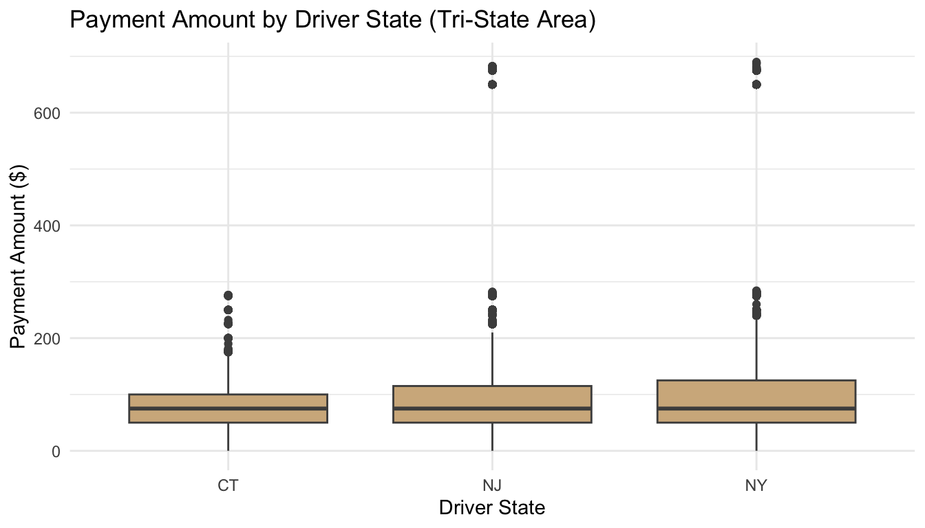
Figure 3.2: Boxplot showing distribution of payment amounts for drivers from the tri-state area (NY, NJ, CT). Highlights differences in payment behavior and variability between states.
3.5.2 Descriptive Statistics
favstats(payment_amount ~ state, data = camera) %>%
  filter(state %in% c("NY","NJ","CT")) %>%
  arrange(desc(mean))
#>   state min Q1 median  Q3    max     mean       sd     n
#> 1    NJ   0 50     75 115 682.35 101.5746 89.97170  8654
#> 2    NY   0 50     75 125 690.04 101.0978 80.92861 79528
#> 3    CT   0 50     75 100 276.57  80.6627 46.07849  1457
#>   missing
#> 1       0
#> 2       0
#> 3       0
3.5.3 Inferential Statistics
tri_state <- camera %>% filter(state %in% c("NY","NJ","CT"))
anova_state <- aov(payment_amount ~ state, data = tri_state)
summary(anova_state)
#>                Df    Sum Sq Mean Sq F value Pr(>F)
#> state           2    603061  301530    45.5 <2e-16 ***
#> Residuals   89636 593994009    6627
#> ---
#> Signif. codes:
#> 0 '***' 0.001 '**' 0.01 '*' 0.05 '.' 0.1 ' ' 1
supernova(anova_state)
#>  Analysis of Variance Table (Type III SS)
#>  Model: payment_amount ~ state
#>
#>                                     SS    df         MS
#>  ----- --------------- | ------------- ----- ----------
#>  Model (error reduced) |    603060.721     2 301530.360
#>  Error (from model)    | 593994008.724 89636   6626.735
#>  ----- --------------- | ------------- ----- ----------
#>  Total (empty model)   | 594597069.446 89638   6633.315
#>       F   PRE     p
#>  ------ ----- -----
#>  45.502 .0010 .0000
#>
#>  ------ ----- -----
#>
3.5.4 Interpretation
A significant p-value (< .05) means payment amounts differ among NY, NJ, and CT drivers.
If out-of-state drivers (NJ or CT) pay more, this could show processing delays or additional penalties.
Even with statistical significance, small PRE values would suggest that differences are limited.
The firm might focus marketing on out-of-state drivers if they tend to pay higher amounts.
3.6 County and Payment Amount
3.6.2 Visualization
ggplot(camera %>% filter(!is.na(county) & county != ""),
       aes(x = county, y = payment_amount)) +
  geom_boxplot(fill = "lightgreen", color = "gray30") +
  coord_flip() +
  theme_minimal() +
  labs(title = "Payment Amount by County",
       x = "County", y = "Payment Amount ($)")
Figure 3.3: Boxplot showing distribution of payment amounts across New York City counties. Helps identifiy geographic patterns in payments and potential focus areas for strategic interventions.
3.6.3 Descriptive Statistics
favstats(payment_amount ~ county, data = camera) %>%
  arrange(desc(mean))
#>             county min  Q1 median     Q3    max      mean
#> 1             RICH 180 180    180 180.00 180.00 180.00000
#> 2  Richmond County   0  65    180 180.00 245.79 139.67920
#> 3            Bronx 115 115    115 115.00 115.00 115.00000
#> 4              Qns 115 115    115 115.00 115.00 115.00000
#> 5               BK   0  50     75 100.00 690.04 113.54971
#> 6    Queens County   0  65    115 125.00 244.46 102.35114
#> 7               MN   0  50     50 125.06 281.80 100.54274
#> 8     Bronx County   0  65     75 160.00 245.64 100.32037
#> 9  New York County   0  65    115 115.00 260.00  92.95323
#> 10    Kings County   0  65     65 115.00 243.81  86.09225
#> 11              QN   0  50     50 100.00 283.03  82.35782
#> 12              ST   0  50     50  75.00 250.00  69.66361
#> 13           Kings   0   0      0   0.00   0.00   0.00000
#>           sd     n missing
#> 1         NA     1       0
#> 2   80.35405   863       0
#> 3         NA     1       0
#> 4         NA     1       0
#> 5  131.50278 14560       0
#> 6   52.58054   983       0
#> 7   73.46670 14518       0
#> 8   67.45720   243       0
#> 9   38.30536  8950       0
#> 10  49.12610  1547       0
#> 11  60.30923 16373       0
#> 12  45.80596   485       0
#> 13        NA     1       0
3.6.4 Inferential Statistics
county_clean <- camera %>% filter(!is.na(county) & county != "")
anova_county <- aov(payment_amount ~ county, data = county_clean)
summary(anova_county)
#>                Df    Sum Sq Mean Sq F value Pr(>F)
#> county         12   9978556  831546   116.7 <2e-16 ***
#> Residuals   58513 416929615    7125
#> ---
#> Signif. codes:
#> 0 '***' 0.001 '**' 0.01 '*' 0.05 '.' 0.1 ' ' 1
supernova(anova_county)
#>  Analysis of Variance Table (Type III SS)
#>  Model: payment_amount ~ county
#>
#>                                     SS    df         MS
#>  ----- --------------- | ------------- ----- ----------
#>  Model (error reduced) |   9978556.010    12 831546.334
#>  Error (from model)    | 416929614.778 58513   7125.419
#>  ----- --------------- | ------------- ----- ----------
#>  Total (empty model)   | 426908170.788 58525   7294.458
#>        F   PRE     p
#>  ------- ----- -----
#>  116.701 .0234 .0000
#>
#>  ------- ----- -----
#> 3.7 Final Summary
Across all analyses, issuing agency, driver state, and county show statistically significant differences in payment amounts, primarily because of the very large dataset.
However, only county likely represents meaningful differences related to enforcement or geographic patterns.
The law firm should prioritize county in its marketing strategy, focusing advertising and outreach in areas with higher average payment amounts.