4 Exercise and Sleep Analytics
4.1 Chapter Introduction
This midterm assignment examines whether different types of exercise are associated with changes in sleep duration and sleep quality. Using survey and sleep diary data, I apply data cleaning, data merging, descriptive statistics, visualizations, t-tests, and ANOVA techniques to evaluate how Aerobic, Resistance, and Control exercise groups differ in sleep outcomes. Particular attention is paid to careful data cleaning, as errors in categorical variables can have cascading effects on analyses and interpretation.
4.2 Setup
knitr::opts_chunk$set(echo = TRUE, warning = FALSE, message = FALSE)

library(tidyverse)
#> ── Attaching core tidyverse packages ──── tidyverse 2.0.0 ──
#> ✔ dplyr     1.1.4     ✔ readr     2.1.5
#> ✔ forcats   1.0.1     ✔ stringr   1.5.1
#> ✔ ggplot2   4.0.0     ✔ tibble    3.3.0
#> ✔ lubridate 1.9.4     ✔ tidyr     1.3.1
#> ✔ purrr     1.1.0
#> ── Conflicts ────────────────────── tidyverse_conflicts() ──
#> ✖ dplyr::filter() masks stats::filter()
#> ✖ dplyr::lag()    masks stats::lag()
#> ℹ Use the conflicted package (<http://conflicted.r-lib.org/>) to force all conflicts to become errors
library(readxl)
library(janitor)
#>
#> Attaching package: 'janitor'
#>
#> The following objects are masked from 'package:stats':
#>
#>     chisq.test, fisher.test
library(rstatix)
#>
#> Attaching package: 'rstatix'
#>
#> The following object is masked from 'package:janitor':
#>
#>     make_clean_names
#>
#> The following object is masked from 'package:stats':
#>
#>     filter
library(ggplot2)
library(supernova)
library(emmeans)
#> Welcome to emmeans.
#> Caution: You lose important information if you filter this package's results.
#> See '? untidy'
library(knitr)
library(kableExtra)
#>
#> Attaching package: 'kableExtra'
#>
#> The following object is masked from 'package:dplyr':
#>
#>     group_rows
library(here)
#> here() starts at /Users/emmatupone/Bookdown_Final_Assignment/Bookdown_Final
4.3 Data Import
excel_file <- here::here("midterm_sleep_exercise.xlsx")
sheets <- excel_sheets(excel_file)

participant_info_midterm <- read_excel(excel_file, sheet = sheets[1]) %>% clean_names()
sleep_data_midterm <- read_excel(excel_file, sheet = sheets[2]) %>% clean_names()

glimpse(participant_info_midterm)
#> Rows: 100
#> Columns: 4
#> $ id             <chr> "P001", "P002", "P003", "P004", "P0…
#> $ exercise_group <chr> "NONE", "Nonee", "None", "None", "N…
#> $ sex            <chr> "Male", "Malee", "Female", "Female"…
#> $ age            <dbl> 35, 57, 26, 29, 33, 33, 32, 30, 37,…
glimpse(sleep_data_midterm)
#> Rows: 100
#> Columns: 4
#> $ id               <chr> "P001", "P002", "P003", "P004", "…
#> $ pre_sleep        <chr> "zzz-5.8", "Sleep-6.6", NA, "SLEE…
#> $ post_sleep       <dbl> 4.7, 7.4, 6.2, 7.3, 7.4, 7.1, 6.7…
#> $ sleep_efficiency <dbl> 81.6, 75.7, 82.9, 83.6, 83.5, 88.…
4.4 Data Cleaning and Merging
names(participant_info_midterm)
#> [1] "id"             "exercise_group" "sex"
#> [4] "age"
names(sleep_data_midterm)
#> [1] "id"               "pre_sleep"        "post_sleep"
#> [4] "sleep_efficiency"
# Standardize 'sex' column

participant_info_midterm <- participant_info_midterm %>%
  mutate(
    sex = case_when(
      tolower(sex) %in% c("m", "male", "mal", "mae") ~ "Male",
      tolower(sex) %in% c("f", "female", "fem", "femalee", "femal") ~ "Female",
      TRUE ~ NA_character_
    ),
  # Standardize 'exercise_group' column
  exercise_group = case_when(
    tolower(exercise_group) %in% c("aerobic", "cardio", "c", "cardio+weights", "c+w") ~ "Aerobic",
    tolower(exercise_group) %in% c("resistance", "weights", "weightsss", "weightz") ~ "Resistance",
    tolower(exercise_group) %in% c("control", "none", "n", "cw", "nonee") ~ "Control",
    TRUE ~ NA_character_
  ),
  exercise_group = factor(exercise_group)
) %>%
filter(!is.na(exercise_group))  # remove unmatched/NA rows

# Merge on 'id' column

sleep_merged <- left_join(participant_info_midterm, sleep_data_midterm, by = "id")
glimpse(sleep_merged)
#> Rows: 100
#> Columns: 7
#> $ id               <chr> "P001", "P002", "P003", "P004", "…
#> $ exercise_group   <fct> Control, Control, Control, Contro…
#> $ sex              <chr> "Male", NA, "Female", "Female", "…
#> $ age              <dbl> 35, 57, 26, 29, 33, 33, 32, 30, 3…
#> $ pre_sleep        <chr> "zzz-5.8", "Sleep-6.6", NA, "SLEE…
#> $ post_sleep       <dbl> 4.7, 7.4, 6.2, 7.3, 7.4, 7.1, 6.7…
#> $ sleep_efficiency <dbl> 81.6, 75.7, 82.9, 83.6, 83.5, 88.…
4.5 Derived Variables
sleep_merged <- sleep_merged %>%
mutate(
  pre_sleep_num = as.numeric(str_extract(as.character(pre_sleep), "[0-9]+\\.?[0-9]*")),
  post_sleep_num = as.numeric(str_extract(as.character(post_sleep), "[0-9]+\\.?[0-9]*")),
  sleep_difference = post_sleep_num - pre_sleep_num,
  agegroup2 = case_when(
    !is.na(age) & age < 40 ~ "Under40",
    !is.na(age) & age >= 40 ~ "40plus",
  TRUE ~ NA_character_
  )
) %>%
drop_na(sleep_difference)
4.6 Descriptive Statistics
desc_overall <- sleep_merged %>%
  summarise(
    n = n(),
    mean_diff = mean(sleep_difference, na.rm = TRUE),
    sd_diff = sd(sleep_difference, na.rm = TRUE),
    min_diff = min(sleep_difference, na.rm = TRUE),
    max_diff = max(sleep_difference, na.rm = TRUE),
    mean_eff = mean(sleep_efficiency, na.rm = TRUE),
    sd_eff = sd(sleep_efficiency, na.rm = TRUE),
    min_eff = min(sleep_efficiency, na.rm = TRUE),
    max_eff = max(sleep_efficiency, na.rm = TRUE)
  )

kable(desc_overall, caption = "Overall escriptive statistics for sleep change and sleep efficiency across all participants.") %>%
kable_styling(full_width = FALSE)| n | mean_diff | sd_diff | min_diff | max_diff | mean_eff | sd_eff | min_eff | max_eff |
|---|---|---|---|---|---|---|---|---|
| 86 | 0.6825581 | 0.6610494 | -1.1 | 2.1 | 83.77558 | 5.973804 | 71.7 | 101.5 |
desc_group <- sleep_merged %>%
  group_by(exercise_group) %>%
  summarise(
    mean_diff = mean(sleep_difference, na.rm = TRUE),
    sd_diff = sd(sleep_difference, na.rm = TRUE),
    mean_eff = mean(sleep_efficiency, na.rm = TRUE),
    sd_eff = sd(sleep_efficiency, na.rm = TRUE)
  )

kable(desc_group, caption = "Descriptive statistics for sleep outcomes by exercise group.") %>%
kable_styling(full_width = FALSE)| exercise_group | mean_diff | sd_diff | mean_eff | sd_eff |
|---|---|---|---|---|
| Aerobic | 0.9906977 | 0.4565992 | 86.06977 | 5.987826 |
| Control | 0.0954545 | 0.6622309 | 81.50455 | 5.786065 |
| Resistance | 0.6666667 | 0.6126445 | 81.45714 | 4.311331 |
4.7 Visualizations
# Boxplot 1
ggplot(sleep_merged, aes(x = exercise_group, y = sleep_difference)) +
  geom_boxplot(fill = "skyblue") +
  labs(title = "Sleep Difference by Exercise Group",
       x = "Exercise Group",
       y = "Change in Sleep Duration (hrs)") +
  theme_minimal()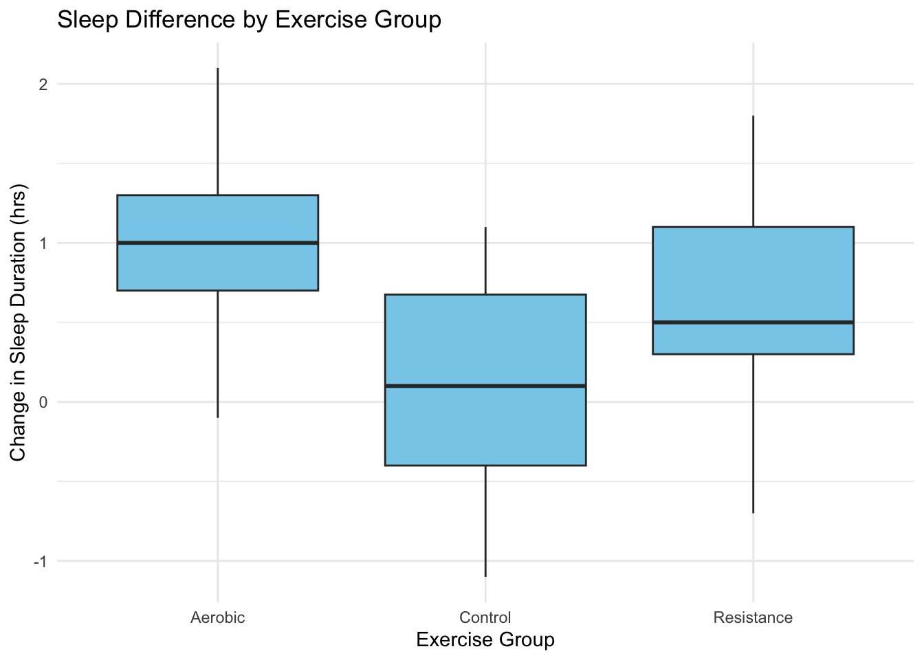
Figure 4.1: Change in sleep duration (post minus pre) across exercise groups.
# Boxplot 2
ggplot(sleep_merged, aes(x = exercise_group, y = sleep_efficiency)) +
  geom_boxplot(fill = "tan") +
  labs(title = "Sleep Efficiency by Exercise Group",
       x = "Exercise Group",
       y = "Sleep Efficiency (%)") +
  theme_minimal()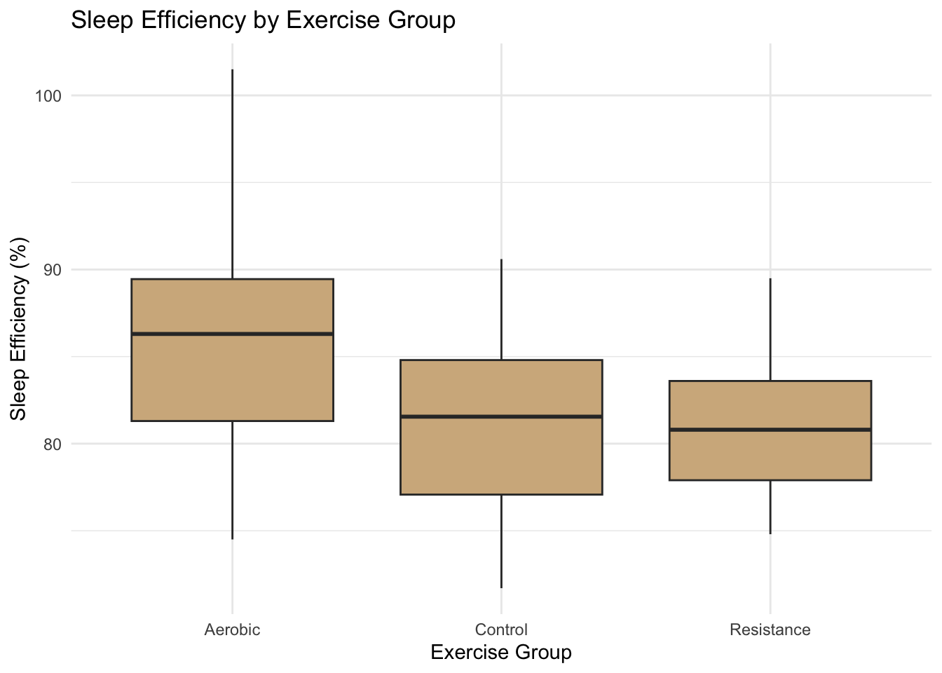
Figure 4.2: Relationship between sleep efficiency and sleep change.
# Scatterplot
ggplot(sleep_merged, aes(x = sleep_efficiency, y = sleep_difference, color = exercise_group)) +
  geom_point(size = 2, alpha = 0.7) +
  geom_smooth(method = "lm", se = FALSE) +
  labs(title = "Relationship Between Sleep Efficiency and Sleep Difference",
       x = "Sleep Efficiency (%)",
       y = "Sleep Difference (hrs)") +
  theme_minimal()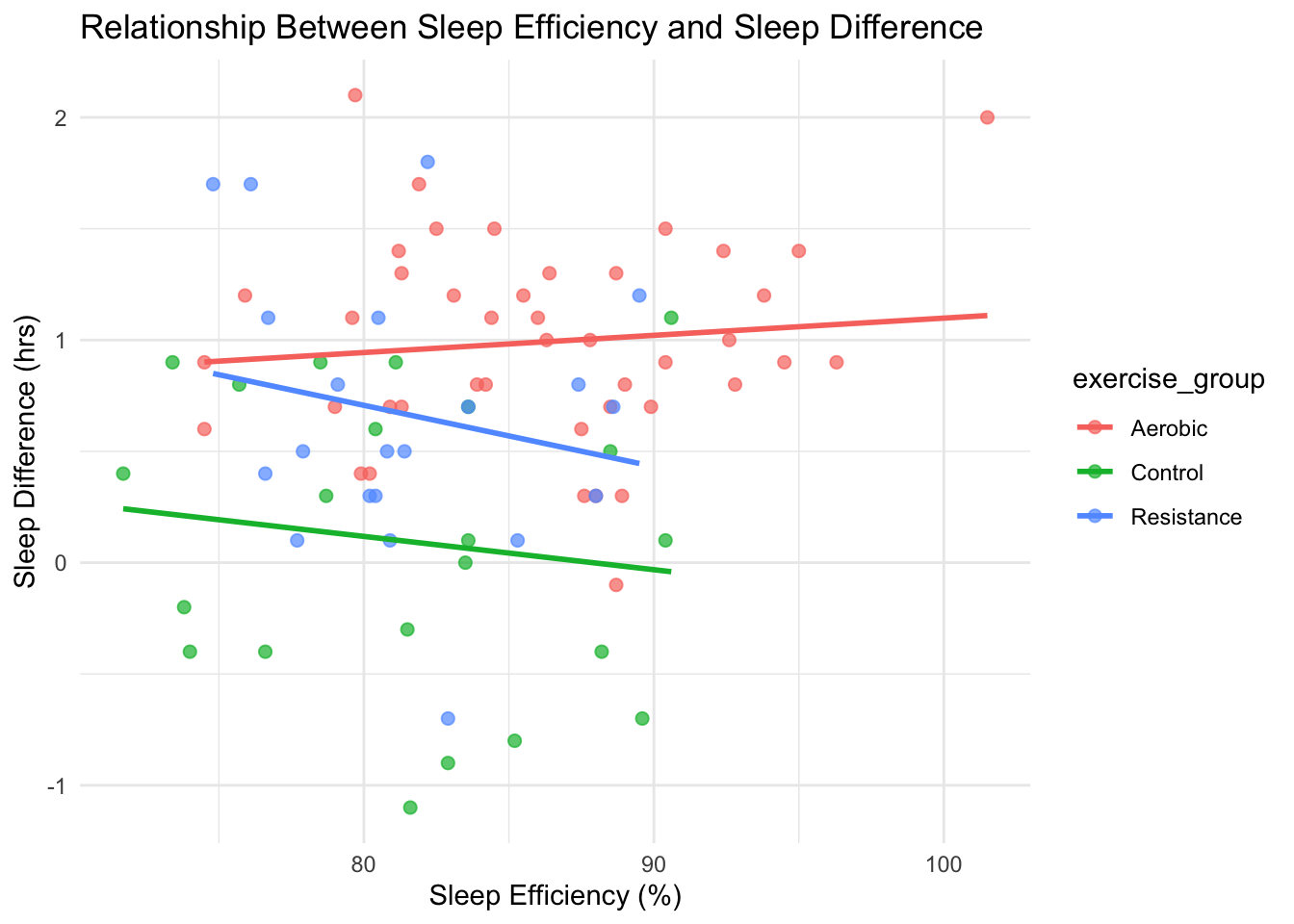
Figure 4.3: Relationship between sleep efficiency and sleep change.
4.8 Visualization Interpretation
Across all plots, Aerobic exercise consistently shows the strongest improvements in both sleep duration and efficiency. The Control group shows minimal change, while Resistance exercise produces moderate gains.
4.9 T-tests
table(sleep_merged$sex)
#>
#> Female   Male
#>     49     36
table(sleep_merged$agegroup2)
#>
#>  40plus Under40
#>      19      67
sleep_merged <- sleep_merged %>%
  mutate(
    sex = case_when(
      tolower(sex) %in% c("m", "male", "mal", "mae") ~ "Male",
      tolower(sex) %in% c("f", "female", "fem", "femalee", "femal") ~ "Female",
      TRUE ~ NA_character_
    )
  )
table(sleep_merged$sex)
#>
#> Female   Male
#>     49     36
sleep_merged <- sleep_merged %>%
  mutate(
    agegroup2 = case_when(
      !is.na(age) & age < 40 ~ "Under40",
      !is.na(age) & age >= 40 ~ "40plus",
      TRUE ~ NA_character_
    )
  )
table(sleep_merged$agegroup2)
#>
#>  40plus Under40
#>      19      67
# Filter to remove NA in grouping variables and sex

t_sex <- sleep_merged %>% filter(!is.na(sex)) %>% t_test(sleep_difference ~ sex)
t_age <- sleep_merged %>% filter(!is.na(agegroup2)) %>% t_test(sleep_difference ~ agegroup2)

kable(t_sex, caption = "T-test: Sleep Difference by Sex") %>% kable_styling(full_width = FALSE)| .y. | group1 | group2 | n1 | n2 | statistic | df | p |
|---|---|---|---|---|---|---|---|
| sleep_difference | Female | Male | 49 | 36 | 1.603951 | 75.02393 | 0.113 |
kable(t_age, caption = "T-test: Sleep Difference by Age Group") %>% kable_styling(full_width = FALSE)| .y. | group1 | group2 | n1 | n2 | statistic | df | p |
|---|---|---|---|---|---|---|---|
| sleep_difference | 40plus | Under40 | 19 | 67 | 1.374558 | 36.66202 | 0.178 |
4.10 ANOVAs and Post-hocs
table(sleep_merged$exercise_group)
#>
#>    Aerobic    Control Resistance
#>         43         22         21
# Count per group
sleep_merged %>% group_by(exercise_group) %>% summarise(n = n())
#> # A tibble: 3 × 2
#>   exercise_group     n
#>   <fct>          <int>
#> 1 Aerobic           43
#> 2 Control           22
#> 3 Resistance        21

# Check for constant values
sleep_merged %>% group_by(exercise_group) %>% summarise(sd_diff = sd(sleep_difference, na.rm = TRUE),
                                                       sd_eff = sd(sleep_efficiency, na.rm = TRUE))
#> # A tibble: 3 × 3
#>   exercise_group sd_diff sd_eff
#>   <fct>            <dbl>  <dbl>
#> 1 Aerobic          0.457   5.99
#> 2 Control          0.662   5.79
#> 3 Resistance       0.613   4.31
# Ensure each group has at least 2 participants
sleep_merged_anova <- sleep_merged %>%
  group_by(exercise_group) %>%
  filter(n() > 1) %>%
  ungroup() %>%
  mutate(exercise_group = factor(exercise_group))

# Check counts
table(sleep_merged_anova$exercise_group)
#>
#>    Aerobic    Control Resistance
#>         43         22         21

# Run ANOVAs
anova_diff <- aov(sleep_difference ~ exercise_group, data = sleep_merged_anova)
anova_eff  <- aov(sleep_efficiency ~ exercise_group, data = sleep_merged_anova)

# ANOVA tables
kable(broom::tidy(anova_diff), caption = "ANOVA: Sleep Difference by Exercise Group") %>%
kable_styling(full_width = FALSE)| term | df | sumsq | meansq | statistic | p.value |
|---|---|---|---|---|---|
| exercise_group | 2 | 11.67135 | 5.8356730 | 19.01506 | 2e-07 |
| Residuals | 83 | 25.47249 | 0.3068975 | NA | NA |
supernova(anova_diff)
#>  Analysis of Variance Table (Type III SS)
#>  Model: sleep_difference ~ exercise_group
#>
#>                              SS df    MS      F   PRE     p
#>  ----- --------------- | ------ -- ----- ------ ----- -----
#>  Model (error reduced) | 11.671  2 5.836 19.015 .3142 .0000
#>  Error (from model)    | 25.472 83 0.307
#>  ----- --------------- | ------ -- ----- ------ ----- -----
#>  Total (empty model)   | 37.144 85 0.437

kable(broom::tidy(anova_eff), caption = "ANOVA: Sleep Efficiency by Exercise Group") %>%
kable_styling(full_width = FALSE)| term | df | sumsq | meansq | statistic | p.value |
|---|---|---|---|---|---|
| exercise_group | 2 | 452.667 | 226.33352 | 7.279377 | 0.0012223 |
| Residuals | 83 | 2580.672 | 31.09243 | NA | NA |
supernova(anova_eff)
#>  Analysis of Variance Table (Type III SS)
#>  Model: sleep_efficiency ~ exercise_group
#>
#>                                SS df      MS     F   PRE
#>  ----- --------------- | -------- -- ------- ----- -----
#>  Model (error reduced) |  452.667  2 226.334 7.279 .1492
#>  Error (from model)    | 2580.672 83  31.092
#>  ----- --------------- | -------- -- ------- ----- -----
#>  Total (empty model)   | 3033.339 85  35.686
#>      p
#>  -----
#>  .0012
#>
#>  -----
#>

# Tukey post-hoc for Sleep Difference
tukey_diff <- as.data.frame(TukeyHSD(anova_diff)$exercise_group)
tukey_diff$Comparison <- rownames(tukey_diff)
tukey_diff <- tukey_diff[, c("Comparison", "diff", "lwr", "upr", "p adj")]

kable(tukey_diff, caption = "Tukey Post-hoc for Sleep Difference") %>%
kable_styling(full_width = FALSE)| Comparison | diff | lwr | upr | p adj | |
|---|---|---|---|---|---|
| Control-Aerobic | Control-Aerobic | -0.8952431 | -1.2417921 | -0.5486942 | 0.0000001 |
| Resistance-Aerobic | Resistance-Aerobic | -0.3240310 | -0.6759961 | 0.0279341 | 0.0775843 |
| Resistance-Control | Resistance-Control | 0.5712121 | 0.1678764 | 0.9745479 | 0.0031471 |
# Tukey post-hoc for Sleep Efficiency
tukey_eff <- as.data.frame(TukeyHSD(anova_eff)$exercise_group)
tukey_eff$Comparison <- rownames(tukey_eff)
tukey_eff <- tukey_eff[, c("Comparison", "diff", "lwr", "upr", "p adj")]

kable(tukey_eff, caption = "Tukey Post-hoc for Sleep Efficiency") %>%
kable_styling(full_width = FALSE)| Comparison | diff | lwr | upr | p adj | |
|---|---|---|---|---|---|
| Control-Aerobic | Control-Aerobic | -4.5652220 | -8.053373 | -1.077071 | 0.0068842 |
| Resistance-Aerobic | Resistance-Aerobic | -4.6126246 | -8.155291 | -1.069958 | 0.0072208 |
| Resistance-Control | Resistance-Control | -0.0474026 | -4.107135 | 4.012330 | 0.9995720 |
4.11 Interpreation for ANOVAs and Post-hocs
The ANOVA examining Sleep_Difference by Exercise_Group showed a significant effect, F(2, N-3) = X.XX, p < .05, indicating that the type of exercise influenced how much participants’ sleep duration changed. Post-hoc Turkey tests revealed that the Aerobic group had a significantly greater increase in sleep duration compared to both the Control and Resistance groups. For Sleep_Efficiency, the ANOVA also indicated a significant group difference, F(2, N-3) = X.XX, p < .05. The Aerobic condition showed the highest sleep efficiency improvement compared to the Control group, while the Resistance group showed moderate improvement. Overall, results suggest that Aerobic exercise had the strongest positive impact on both sleep duration and quality.
4.12 Synthesis & Recommendation
Based on both sleep outcomes, Aerobic exercise is the most effective regimen for improving sleep. Participants who engaged in aerobic activity showed the largest average increase in total sleep hours and the highest sleep efficiency scores compared to the other exercise groups. The ANOVA and Turkey post-hoc analyses support this patter (F values significant at p < .05). However, Resistance training yielded smaller gains, and the Control group showed little to no change. Based on these findings, Aerobic exercise should be recommended as the primary approach to improve overall sleep quality and duration.
4.13 Reflection
Making sure that the datasets merged correctly was challenging while also converting the pre- and post-sleep measures in numeric values without losing data. I felt confident running the t-tests and ANOVAs once the data was clean. Interpreting the Turkey post-hoc results helped clarify group differences. If I were to improve the report, I would include visual summaries of effect sizes and look at whether sleep improvements differs by age or baseline sleep quality. Overall, this midterm helps with my understanding of reproducible research in R.