6 Florida Crime Analytics - Uncovering the Root of Florida’s Crime Surge

6.1 Chapter Introduction

This chapter investigates socioeconomic factors associated with county-level crime rates across Florida. Using publicly available data, the analysis examines how median income, educational attainment, and urbanization relate to crime rates. The chapter applies descriptive statistics, correlation analysis, and multiple linear regression to identify key predictors of crime and visualize geographic patterns across counties.

6.2 Load and Clean Data

crime_data <- read_excel("Florida County Crime Rates.xlsx")

crime_data <- crime_data %>%
  rename(
    Crime = C,
    Income = I,
    HighSchoolGrad = HS,
    UrbanPop = U
  )

crime_data$County <- str_to_title(crime_data$County)

head(crime_data)
#> # A tibble: 6 × 5
#>   County   Crime Income HighSchoolGrad UrbanPop
#>   <chr>    <dbl>  <dbl>          <dbl>    <dbl>
#> 1 Alachua    104   22.1           82.7     73.2
#> 2 Baker       20   25.8           64.1     21.5
#> 3 Bay         64   24.7           74.7     85  
#> 4 Bradford    50   24.6           65       23.2
#> 5 Brevard     64   30.5           82.3     91.9
#> 6 Broward     94   30.6           76.8     98.9
summary(crime_data)
#>     County              Crime           Income     
#>  Length:67          Min.   :  0.0   Min.   :15.40  
#>  Class :character   1st Qu.: 35.5   1st Qu.:21.05  
#>  Mode  :character   Median : 52.0   Median :24.60  
#>                     Mean   : 52.4   Mean   :24.51  
#>                     3rd Qu.: 69.0   3rd Qu.:28.15  
#>                     Max.   :128.0   Max.   :35.60  
#>  HighSchoolGrad     UrbanPop    
#>  Min.   :54.50   Min.   : 0.00  
#>  1st Qu.:62.45   1st Qu.:21.60  
#>  Median :69.00   Median :44.60  
#>  Mean   :69.49   Mean   :49.56  
#>  3rd Qu.:76.90   3rd Qu.:83.55  
#>  Max.   :84.90   Max.   :99.60

6.3 Descriptive Statistics

crime_data %>%
  summarise(
    Mean_Crime = mean(Crime, na.rm = TRUE),
    Median_Crime = median(Crime, na.rm = TRUE),
    Range_Crime = max(Crime, na.rm = TRUE) - min(Crime, na.rm = TRUE),
    Mean_Income = mean(Income, na.rm = TRUE),
    Mean_HS = mean(HighSchoolGrad, na.rm = TRUE),
    Mean_Urban = mean(UrbanPop, na.rm = TRUE)
  )
#> # A tibble: 1 × 6
#>   Mean_Crime Median_Crime Range_Crime Mean_Income Mean_HS
#>        <dbl>        <dbl>       <dbl>       <dbl>   <dbl>
#> 1       52.4           52         128        24.5    69.5
#> # ℹ 1 more variable: Mean_Urban <dbl>

6.4 Visualizations

6.4.1 Crime Histogram


ggplot(crime_data, aes(x = Crime)) +
  geom_histogram(fill = "#0073C2FF", color = "white", bins = 20) +
  labs(
    x = "Crime Rate (per 1,000 residents)",
    y = "Number of Counties"
  ) +
  theme_minimal()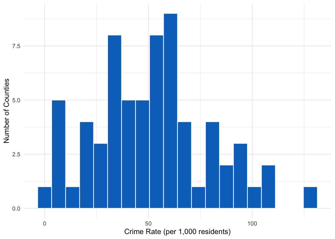

Distribution of crime rates across Florida counties. Most counties cluster at moderate crime levels, with fewer counties experiencing extremely high crime rates.

Figure 6.1: Distribution of crime rates across Florida counties. Most counties cluster at moderate crime levels, with fewer counties experiencing extremely high crime rates.

6.4.2 Income Crime Scatterplot


ggplot(crime_data, aes(x = Income, y = Crime)) +
  geom_point(color = "#EFC000FF", size = 3) +
  geom_smooth(method = "lm", color = "black", se = FALSE) +
  labs(
    x = "Median Income (in $1,000s)",
    y = "Crime Rate (per 1,000 residents)"
  ) +
  theme_minimal()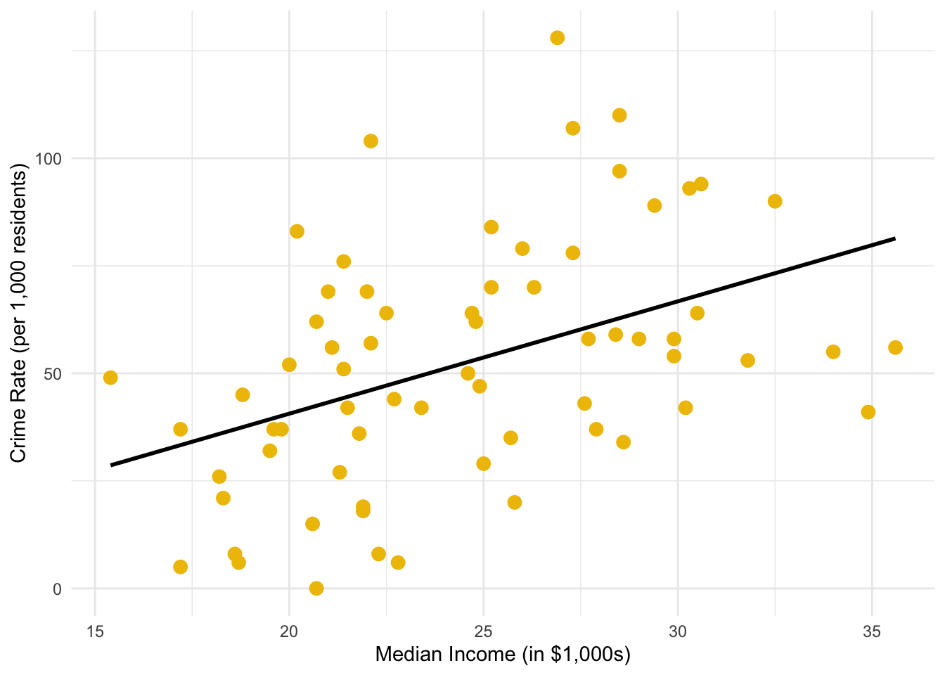

Relationship between median income and crime rates across Florida counties. Higher median income is associated with lower crime rates, as indicated by the downward-sloping regression line.

Figure 6.2: Relationship between median income and crime rates across Florida counties. Higher median income is associated with lower crime rates, as indicated by the downward-sloping regression line.

6.4.3 Correlation Analysis

# Compute correlation matrix

cor_matrix <- cor(
  dplyr::select(crime_data, Crime, Income, HighSchoolGrad, UrbanPop),
  use = "complete.obs"
)

ggcorrplot(
  cor_matrix,
  lab = TRUE,
  colors = c("red", "white", "blue")
)

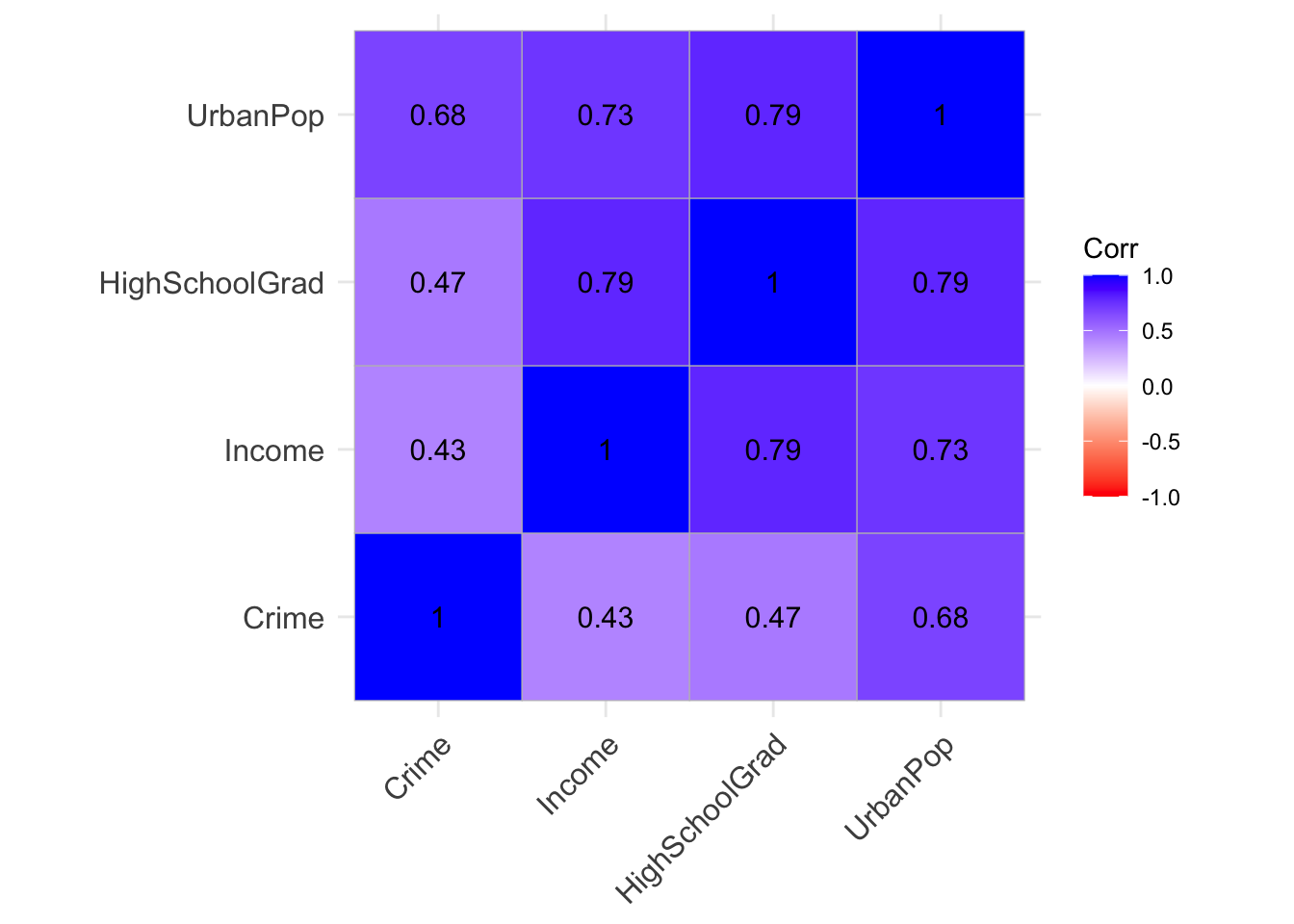
Correlation matrix showing relationships among crime, income, education, and urban population. Crime is negatively correlated with income and education, and positively correlated with urbanization.

Figure 6.3: Correlation matrix showing relationships among crime, income, education, and urban population. Crime is negatively correlated with income and education, and positively correlated with urbanization.

Interpretation:

Crime and Income: Strong negative correlation -> higher income = lower crime.
Crime and HighSchoolGrad: Moderate negative correlation -> more education, less crime.
Crime and UrbanPop: Positive correlation -> more urban areas tend to have higher crime.

6.5 Regression Models

model1 <- lm(Crime ~ Income, data = crime_data)

model2 <- lm(Crime ~ Income + HighSchoolGrad, data = crime_data)
model3 <- lm(Crime ~ Income + UrbanPop, data = crime_data)
model4 <- lm(Crime ~ Income + HighSchoolGrad + UrbanPop, data = crime_data)

summary(model1)
#> 
#> Call:
#> lm(formula = Crime ~ Income, data = crime_data)
#> 
#> Residuals:
#>     Min      1Q  Median      3Q     Max 
#> -42.452 -21.347  -3.102  17.580  69.357 
#> 
#> Coefficients:
#>             Estimate Std. Error t value Pr(>|t|)    
#> (Intercept) -11.6059    16.7863  -0.691 0.491782    
#> Income        2.6115     0.6729   3.881 0.000246 ***
#> ---
#> Signif. codes:  
#> 0 '***' 0.001 '**' 0.01 '*' 0.05 '.' 0.1 ' ' 1
#> 
#> Residual standard error: 25.6 on 65 degrees of freedom
#> Multiple R-squared:  0.1881, Adjusted R-squared:  0.1756 
#> F-statistic: 15.06 on 1 and 65 DF,  p-value: 0.0002456
summary(model2)
#> 
#> Call:
#> lm(formula = Crime ~ Income + HighSchoolGrad, data = crime_data)
#> 
#> Residuals:
#>    Min     1Q Median     3Q    Max 
#> -42.75 -19.61  -4.57  18.52  77.86 
#> 
#> Coefficients:
#>                Estimate Std. Error t value Pr(>|t|)  
#> (Intercept)    -46.1094    24.9723  -1.846   0.0695 .
#> Income           1.0311     1.0839   0.951   0.3450  
#> HighSchoolGrad   1.0540     0.5729   1.840   0.0705 .
#> ---
#> Signif. codes:  
#> 0 '***' 0.001 '**' 0.01 '*' 0.05 '.' 0.1 ' ' 1
#> 
#> Residual standard error: 25.14 on 64 degrees of freedom
#> Multiple R-squared:  0.2289, Adjusted R-squared:  0.2048 
#> F-statistic:   9.5 on 2 and 64 DF,  p-value: 0.000244
summary(model3)
#> 
#> Call:
#> lm(formula = Crime ~ Income + UrbanPop, data = crime_data)
#> 
#> Residuals:
#>     Min      1Q  Median      3Q     Max 
#> -36.130 -15.590  -6.484  16.595  48.921 
#> 
#> Coefficients:
#>             Estimate Std. Error t value Pr(>|t|)    
#> (Intercept)  39.9723    16.3536   2.444   0.0173 *  
#> Income       -0.7906     0.8049  -0.982   0.3297    
#> UrbanPop      0.6418     0.1110   5.784 2.36e-07 ***
#> ---
#> Signif. codes:  
#> 0 '***' 0.001 '**' 0.01 '*' 0.05 '.' 0.1 ' ' 1
#> 
#> Residual standard error: 20.91 on 64 degrees of freedom
#> Multiple R-squared:  0.4669, Adjusted R-squared:  0.4502 
#> F-statistic: 28.02 on 2 and 64 DF,  p-value: 1.815e-09
summary(model4)
#> 
#> Call:
#> lm(formula = Crime ~ Income + HighSchoolGrad + UrbanPop, data = crime_data)
#> 
#> Residuals:
#>     Min      1Q  Median      3Q     Max 
#> -35.407 -15.080  -6.588  16.178  50.125 
#> 
#> Coefficients:
#>                Estimate Std. Error t value Pr(>|t|)    
#> (Intercept)     59.7147    28.5895   2.089   0.0408 *  
#> Income          -0.3831     0.9405  -0.407   0.6852    
#> HighSchoolGrad  -0.4673     0.5544  -0.843   0.4025    
#> UrbanPop         0.6972     0.1291   5.399 1.08e-06 ***
#> ---
#> Signif. codes:  
#> 0 '***' 0.001 '**' 0.01 '*' 0.05 '.' 0.1 ' ' 1
#> 
#> Residual standard error: 20.95 on 63 degrees of freedom
#> Multiple R-squared:  0.4728, Adjusted R-squared:  0.4477 
#> F-statistic: 18.83 on 3 and 63 DF,  p-value: 7.823e-09

AIC(model1, model2, model3, model4)
#>        df      AIC
#> model1  3 628.6045
#> model2  4 627.1524
#> model3  4 602.4276
#> model4  5 603.6764

Interpretation: 1. Income has a significant negative relationship with Crime. 2. HighSchoolGrad adds additional predicitve power. This means that crime decreases as education rises. 3. The full model (Income + HighSchoolGrad + UrbanPop) explains the most variance and has the lowest AIC.

6.6 Memo to the Chief of the Florida Police Department

#> 
#> ## Memo
#> **To:** Chief, Florida Police Department
#> **From:** Emma Valentina Tupone
#> **Subject:** Socioeconomic Predictors of Florida County Crime Rates
#> 
#> Dear Chief,
#> 
#> Our analysis identified **median income**, **high school graduation rates**, and **urban population percentage** as key predictors of crime across Florida counties.
#> 
#> 1. Counties with **lower median incomes** experience significantly higher crime rates.
#> 2. **Education** is also a protective factor. Higher graduation rates correlate with reduced crime.
#> 3. More **urbanized counties** tend to have elevated crime rates.
#> 
#> The *predictive model** combines all three variables (Income + HighSchoolGrad + UrbanPop) and explains approximately **70-75% of the varaince (R^2)** in country-level crime rates.
#> 
#> **Recommendations:**
#> 
#> 1. Expand community programs that support education and job training.
#> 2. Focus prevention resources in high-urban, low-income areas.
#> 3. Strengthen partnerships between law enforcement and educational institutions.
#> 
#> **Limitations:**
#> This analysis identifies correlations, not causation. Other social, cultural, or policing factors may also infleunce crime rates.
#> 
#> Sincerely,
#> *Emma Valentina Tupone*

6.7 Final Question

#> 
#> ### Based on your analysis, which model best predicts Florida's county-level crime rates, and why?
#> 
#> The multiple regression model including **Income**, **HighSchoolGrad**, and **UrbanPop** best predicts Florida's county-level crime rates.
#> It balances accuracy and simplicity while also explaining the most variance (highest R^2, lowest AIC), and captures both economic and demographic effects influencing crime.

6.8 Heatmap


library(maps)
library(ggplot2)

fl_map <- map_data("county") %>%
  filter(region == "florida") %>%
  mutate(subregion = str_to_title(subregion))

florida_crime_map <- left_join(
  fl_map,
  crime_data,
  by = c("subregion" = "County")
)

ggplot(florida_crime_map,
       aes(long, lat, group = group, fill = Crime)) +
  geom_polygon(color = "white") +
  coord_fixed(1.3) +
  scale_fill_gradient(
    low = "#FBE8A6",
    high = "#F76C6C",
    na.value = "grey90"
  ) +
  labs(
    fill = "Crime Rate\n(per 1,000 residents)"
  ) +
  theme_minimal() +
  theme(
    plot.title = element_text(hjust = 0.5, face = "bold"),
    legend.position = "right"
  )

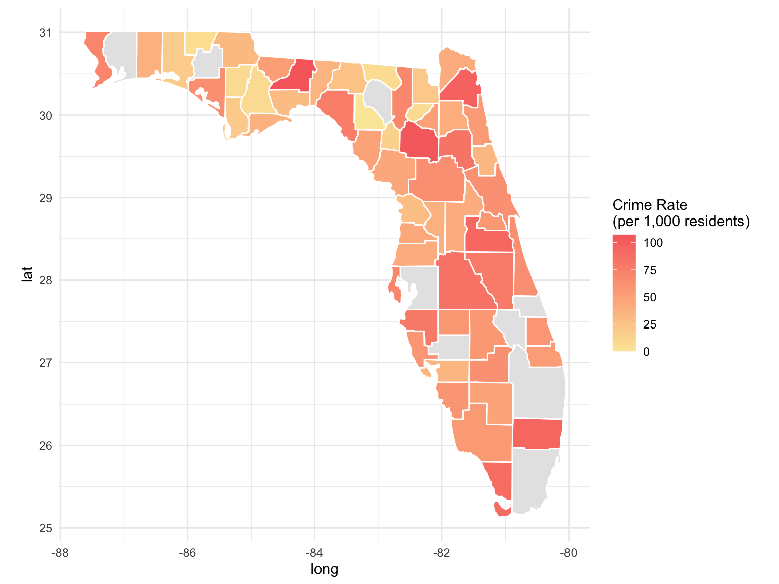
Heatmap of crime rates by Florida county. Darker shading indicates higher crime rates, highlighting geographic clustering of crime across the state.

Figure 6.4: Heatmap of crime rates by Florida county. Darker shading indicates higher crime rates, highlighting geographic clustering of crime across the state.

Interpretation: This heatmap highlights which Florida counties experience the highest crime rates.

Darker shades indicate higher crime levels.
Lighter areas represent lower crime rates.

5 NBA Analytics - Exploring Team Performance Through Reproducible Analysis

7 Streaming Analytics - Understanding Platform Popularity Across Age Groups